Got feedback? Additional questions? Just want to have a friendly chat?
Get in touch!
Prerequisites
Before starting the analysis:
-
A precomputed origin destination time series data set must be configured.
-
The data set must define origin and destination properties.
Opening the origin destination analysis dialog
To open the origin destination analysis:
-
Open the visual analytics page.
-
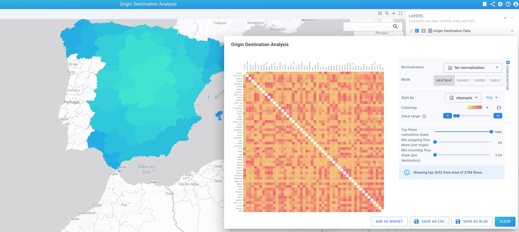
Open the Origin Destination dialog from the Layer Panel. The origin destination icon (a matrix icon) can be found next to the layer name.
The dialog loads the analysis visualization and styling controls.
The different origin destination analysis options
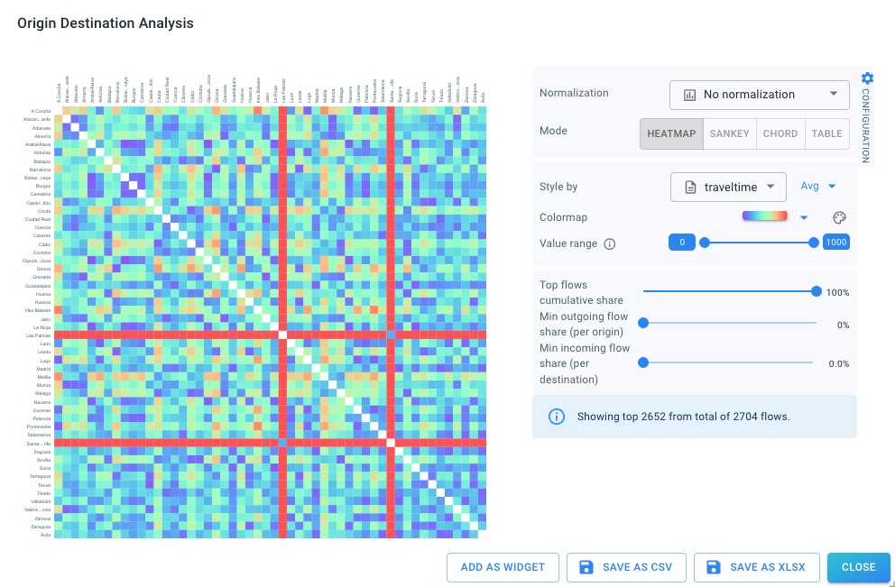
Heatmap
The heatmap visualizes the full origin destination matrix as a grid.
Each cell represents a single origin–destination pair and is colored based on the selected metric. This view is useful for identifying patterns, clusters, and asymmetries.
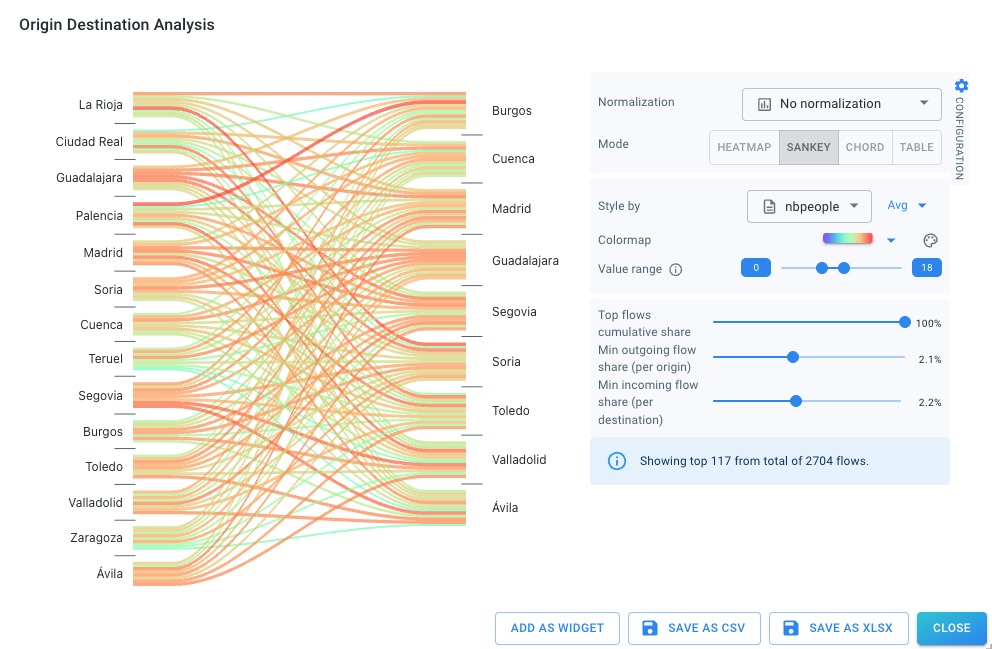
Sankey
The Sankey diagram visualizes flows from origins to destinations using weighted links.
It is useful for identifying dominant flows and understanding how outgoing traffic from origins is distributed across destinations.
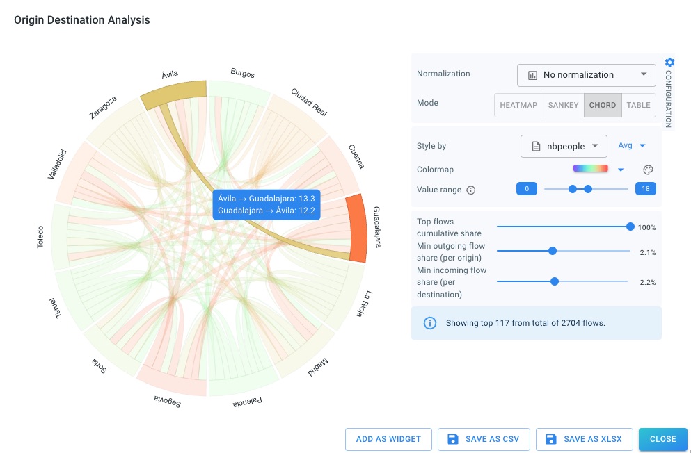
Chord
The chord diagram arranges origins and destinations around a circle and connects them with weighted arcs.
This view is useful for exploring mutual relationships and bidirectional flows.
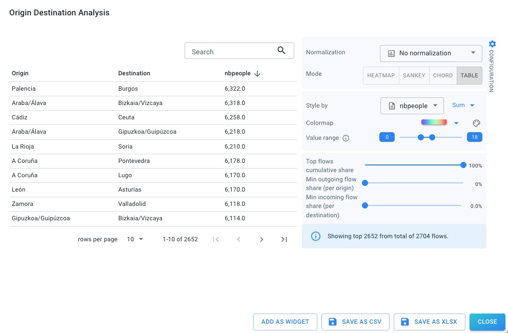
Table
The table view lists all origin destination pairs with their values.
It is useful for sorting, inspecting exact values, and exporting results.
Styling and filtering
Styling and value range
You can choose which numeric attribute is used for styling and whether values are aggregated using sum or average.
The color map and value range can be adjusted to focus on relevant value intervals.
Styling of the origin destination diagrams (heatmap, Sankey,…) is independent of the styling of the map layer.
Filtering
Filtering for precomputed origin destination time series is performed through the corresponding layer filters on the Visual Analytics page.
All filters apply directly to the underlying time series records before the origin destination visualization is computed.
Filtering by origin and destination
The origin ID and destination ID properties behave like regular categorical properties and can be used in filters:
-
Filtering on an origin ID restricts the analysis to records that start in the selected origin.
-
Filtering on a destination ID restricts the analysis to records that end in the selected destination.
-
Combining both filters restricts the analysis to a single origin–destination pair (albeit over multiple time periods).
The effect of these filters is consistent across all origin destination visualizations (heatmap, Sankey, chord, and table).
Filtering with additional ID property
If the precomputed O-D time series includes an additional ID property, filtering behaves slightly differently:
-
An origin ID filter selects trips starting at the chosen origin.
-
A destination ID filter further restricts the selection to trips ending at the chosen destination.
-
The additional ID is interpreted as an intermediate geometry:
-
the analysis aggregates values for trips that pass through the rendered geometry
-
and do so within the active temporal filter range
-
This allows you to analyze how flows propagate through intermediate areas, not just at their origins and destinations.
Temporal and value-based filtering
In addition to origin and destination filters, you can also apply:
-
Temporal filters to restrict the analysis to a specific time window
-
Value-based filters (e.g. minimum number of trips, travel time thresholds)
-
Other categorical or numeric filters present in the data set
All filters are applied before aggregation, ensuring that the resulting origin destination visualizations reflect only the selected subset of data.
Creating widgets and exporting data
From the Origin Destination dialog, you can:
-
Add as widget to add the current analysis as a widget on the project dashboard
-
Save as CSV to export the underlying results
-
Save as XLSX to export to an Excel-compatible format
Got feedback? Additional questions? Just want to have a friendly chat?
Get in touch!