Introduction
The trend analytics page shows histograms: on one axis the time is plotted while the other shows the value.
This value is calculated by looping over the records in your data set that match the configured filter, assigning them to a time bucket and converting the records in each of those time buckets into a single value.
There are multiple ways to do this conversion from records to a single value. This article describes them in more detail, and how you can influence them.
Properties: record versus asset-based calculations
The calculation of the histogram of a property of the data (for example the speed of vehicles over time) can be done on the level of the individual records or the assets.
Asset based calculations
When performing the calculations on an asset-based level, the retained records after filtering for each bucket:
-
Are first grouped by asset
-
For each asset, a value is calculated based on the records of that asset. For example, the min, max or average value
-
This results in a value for each asset. Those values are aggregated into a single value for the bucket, for example by calculating the average.
See Customizing the calculation mode on how to customize both aggregations.
Record based calculations
When performing the calculations on a record-based level, the retained records after filtering for each bucket are directly aggregated into a single value for the bucket.
See Customizing the calculation mode on how to customize this aggregation.
Asset/record counts
For assets and record counts, the calculations inside a single bucket are pre-defined and cannot be customized.
-
Asset count: the value of a single bucket is determined by the number of assets in the bucket
-
Record count: the value of a single bucket is determined by the number of records in the bucket
Group by hour/day/month
When the platform calculates a histogram grouped by hour/day/month, there are two different ways to do this grouping.
Calculate first, group later
In this option, the calculation starts with a continuous time axis and only groups all matching hours/days/months together afterward.
Let’s look at an example where the period of the histogram spans 2 weeks and group by day is chosen. This means that there are 2 Mondays, 2 Tuesdays, … in the data.
In this mode the platform will:
-
Create a time axis with 14 buckets (Monday to Sunday of week 1 and Monday to Sunday of week 2)
-
Assign the filtered records to their corresponding bucket, and calculate a value for each bucket. This calculation is done as described in the previous sections of this article.
-
Once there is a value for each bucket, the 2 Monday buckets are grouped together into a single Monday bucket. The 2 values are aggregated into a single value for the resulting Monday bucket, for example by taking the average.
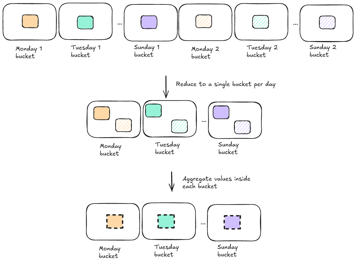
Group up front
In this calculation, only the buckets that will be present in the final histogram are used.
Let’s look at an example where the period of the histogram spans 2 weeks and group by day is chosen. This means that there are 2 Mondays, 2 Tuesdays, … in the data.
In this mode the platform will:
-
Create a time axis with just 7 buckets (Monday to Sunday)
-
Assign the filtered records to their corresponding bucket
-
For each of those buckets, calculate a single value. This calculation is done as described in the previous sections of this article.
Customizing the calculation mode
Regular trends
Currently, the platform only offers limited calculation customizations for regular trends.
For properties, the platform uses the Asset based calculations strategy. There is one UI element available to select an aggregation mode, and this aggregation mode will be used for both the aggregation of record values into asset values and the aggregation of asset values into a bucket value.
When the time axis of the histogram is grouped by hour/day/month, the platform uses the Calculate first, group later strategy. The multiple bucket values are aggregated into a single value using the average.
Categorized trends
The categorized trends page offers options in the UI to customize all the available calculation options.


