Got feedback? Additional questions? Just want to have a friendly chat?
Get in touch!
|
This article only applies to movement data
This article is only relevant when working with movement data, not when working with time series data. You can read more about the differences between the two in this article. |
What is it ?
To maintain scalability and interactivity, during analysis you don’t work with the raw input data but rather with a processed version.
During this processing, the world is divided into cells and the location of your records is mapped onto such a spatial cell. When multiple locations are recorded for the same asset (ship, car, person, …) in a too short amount of time, certain recordings will be dropped.
For example, if your input data specifies the following location for an asset
-
Longitude: 10.23457575
-
Latitude: 15.576835475
after processing, this will be simplified to
-
Location: somewhere in the spatial cell with goes from longitude 10 to 11 degrees, and latitude 15 to 16 degrees
If almost immediately afterwards a second location is recorded for that same asset, that second recording is simply ignored.
You can configure
-
the size of these spatial cells
-
the time delta between 2 recordings of the same asset for which the second recording gets ignored
The remainder of this article explains both the spatial and temporal aggregation in more detail, and illustrates how you can configure these settings for your data sets.
How to configure it ?
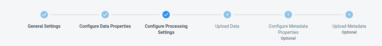
When you are creating or editing a data set, click the Configure Processing Settings button:
Figure 1. The Configure processing settings button in the top navigation bar when creating/editing a data set
On this page, you can fill in the spatial and temporal resolution.
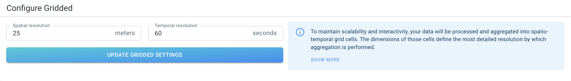
Figure 2. The UI to adjust the spatial and temporal resolution
-
The spatial resolution is expressed in meters
-
The temporal resolution is expressed in seconds
|
You can always adjust the resolution
even when data has already been processed. The only caveat is that adjusting these settings requires the data set to be processed again. This takes some time. |
Details on the spatial resolution
The spatial resolution defines the most detailed resolution by which aggregation on the data is performed. For example, setting this to 500 (meters) means that data points are aggregated in cells of up to 500m x 500m.
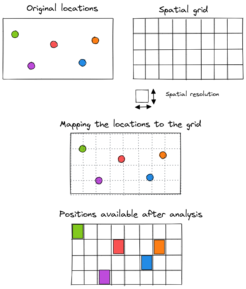
Figure 3. Illustration of how the spatial resolution affects the location available during analysis
Taking a too large value here (e.g., 1000000 (meters)) means that you cannot distinguish between individual location records, as all records within a 1000km range will be aggregated to a single cell.
Taking a too small value here (e.g., 0.01 (meters)) means that, at the most detailed level, cells of 1cm x 1cm will be created, resulting in possible long processing time and larger disk storage.
As a general rule, the resolution should be related to the accuracy of your data and/or the resolution of the analysis you want to perform:
-
Outdoor GPS data: 1-100 (meters) are reasonable values.
-
Indoor Bluetooth data: 0.5-10 (meters) are reasonable values.
Figure 4. When zoomed out, the spatial grid is hardly visible
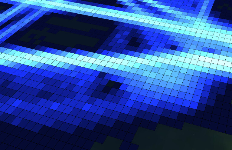
Figure 5. When zooming in to the most detailed level, the spatial tiles become visible
Details on the temporal resolution
The temporal resolution defines the temporal ‘spread’ of a discrete record. When two recordings of the same asset fall in the same cell, this temporal resolution is used to determine whether the record is counted once or twice.
Let’s look at an example to clarify this. Assume you have a data set containing the positions of ships. If you have 2 recordings of the position of the same ship, and these 2 recordings:
-
place the vessel in the same spatial cell
-
and the time difference between those 2 recordings is smaller than the temporal resolution
the second recording will be ignored.
The second recording is only excluded when both conditions (same cell and time difference smaller than the temporal resolution) are met.
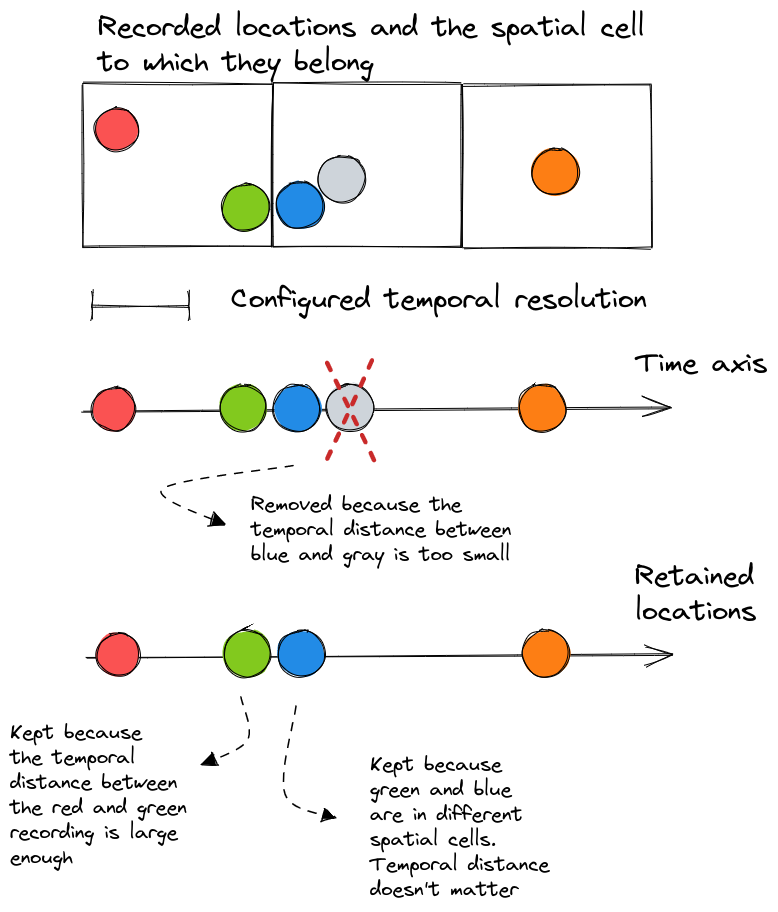
Figure 6. Illustration of how the temporal resolution affects which recordings are considered during analysis
Overview levels
When you configure the spatial and temporal resolution, the values you provide will be used on the most detailed level which becomes visible when you zoom in all the way.
Once you started zooming out on the spatial map, data from less-detailed levels or overview levels will be loaded. For each new overview level, both the spatial and temporal resolution are doubled.
-
First overview level:
-
Spatial resolution = 2 * configured spatial resolution
-
Temporal resolution = 2 * configured temporal resolution
-
-
Second overview level:
-
Spatial resolution = 4 * configured spatial resolution
-
Temporal resolution = 4 * configured temporal resolution
-
-
Third overview level:
-
Spatial resolution = 8 * configured spatial resolution
-
Temporal resolution = 8 * configured temporal resolution
-
-
…
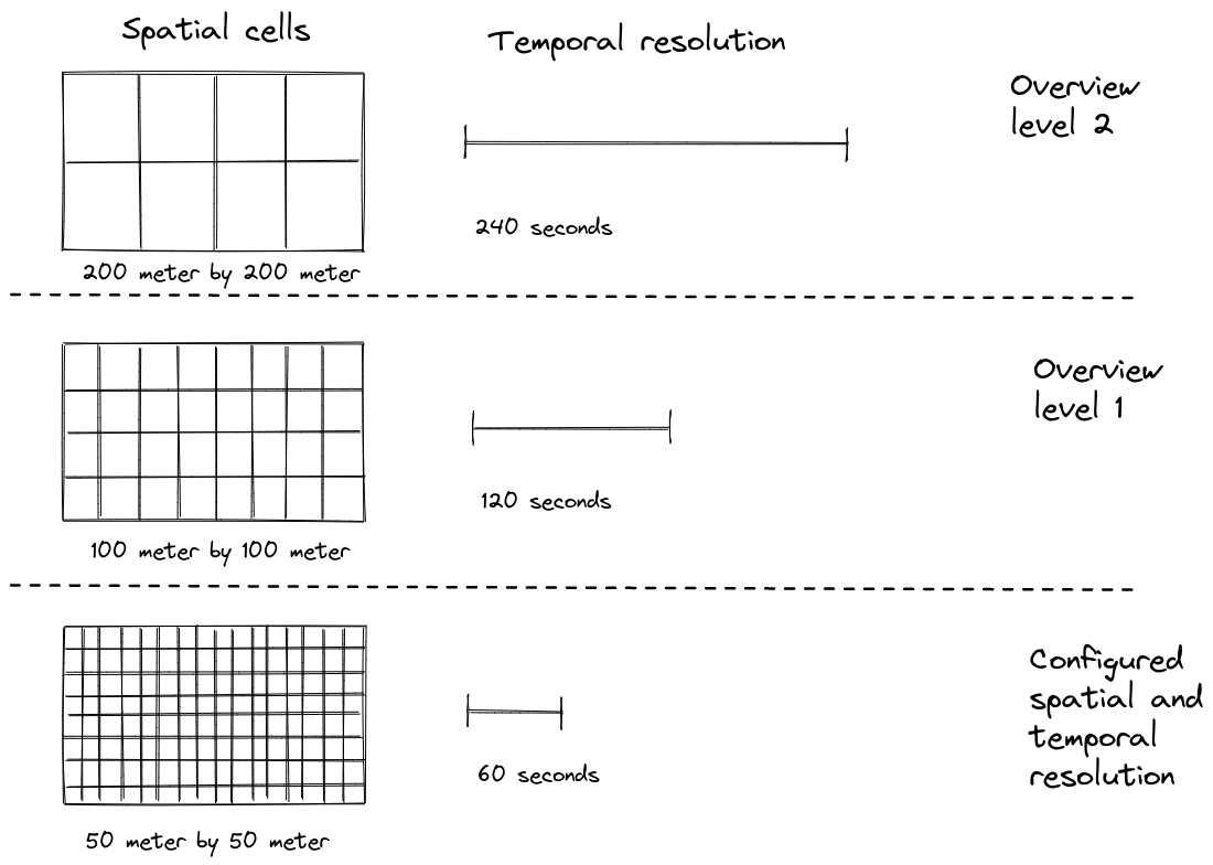
Figure 7. Overview of how the spatial and temporal resolution change on the different overview levels
Got feedback? Additional questions? Just want to have a friendly chat?
Get in touch!