Introduction
Travel time is, as the word implies, the time it takes an asset to travel between a start and end location.
This travel time can be used on:
-
The timeline on the visual analytics page
-
The trend analytics pages (both regular and categorized)
-
The distribution analytics pages
Working with travel times in the platform is the same as working with other properties from your data.
When the platform needs to calculate something (e.g. a histogram, a distribution, a spatial tile, …), it always goes through a 2-step process:
-
Find the relevant records by looping over the data and applying the configured filter. This results in a set of retained records.
-
Those records are then used to calculate the requested histogram or distribution. This involves either counting the records/assets, or extracting a property (e.g. the speed) from a record. More details about this are available in dedicated articles, for example this article describes the calculation for histograms.
In this regard, travel time can be seen as a metadata property. Once the filter has been evaluated, the records passed into the histogram/distribution/… calculation have an extra "travel-time" property that the calculation could use. It is similar to a metadata property because the value of the property is the same for each record of an asset.
As such, these calculations can use the travel time just like any other metadata property.
Calculation of the travel time
To understand this section, you need to know the different kind of filters the platform offers.
There are 3 scenarios for the calculation of travel times:
Without an asset route filter
When there is no asset route filter, the travel time is the time difference between the last known record of the asset and the first known record of the asset in the whole data set.
This last part is important to remember.
For example if you have an asset that travels from A → B → C → D, the travel time when no asset route filter is specified will always be the time to travel from A → D. Even when you use a record filter to only retain the records in area B, the travel time will still be the time it took to travel from A to D because the travel time calculation only looks at the asset route filter.
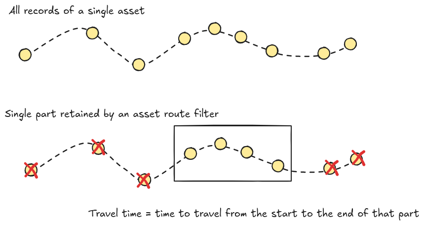
With an asset route filter with a single matching segment
An asset route filter only retains one or more continuous parts of the trajectory of an asset.
Assume that the asset route filter retains one continuous part of the asset. In this case, the travel time is defined as the time for the asset to travel that part of the route.
With an asset route filter with multiple matching segments
An asset route filter only retains one or more continuous parts of the trajectory of an asset.
In case the asset route filter retains multiple parts of the asset’s trajectory, there is no single travel time but rather a travel time per part of the trajectory. As such, the travel time exposed on the records is not constant either. Instead, it is constant for all the records belonging to the same part of the asset’s trajectory.
For example, suppose the asset route filter retained 2 parts of the asset’s trajectory:
-
One part with a travel time of 3 hours, consisting of 10 records
-
One part with a travel time of 5 hours, consisting of 20 records
The travel time for the 10 records of the first part will be 3 hours, and the travel time associated with the records of the second part is 5 hours.
Filtering on travel times
You can use the DURATION retrieval function to access the travel time,
and use this in an asset filter.
An example use case for this is filtering out outliers from your data.
Suppose you want to analyze the travel times from Brussels to Leuven using the following filter:
ASSET_ROUTE(
  INSIDE(LOC(), AREA(name="Brussels")),
  ANY(),
  INSIDE(LOC(), AREA(name="Leuven"))
)
Typically, these are under one hour but your data set might contain some outliers, for example somebody who started in Brussels, drove to the shop to do grocery shopping, and only then continued to Leuven.
You could filter out such outliers by limiting your analysis to travel times of maximum one hour:
ASSET_ROUTE(
  INSIDE(LOC(), AREA(name="Brussels")),
  ANY(),
  INSIDE(LOC(), AREA(name="Leuven"))
) |
ASSET(
  LTE(
    DURATION(), 3600
  )
)