Got feedback? Additional questions? Just want to have a friendly chat?
Get in touch!
Available parts
- Goal
- Roadworks, traffic diversions, and floating vehicle data
- Setting up a traffic flow analysis project
- Analzying traffic flows using basic filters
- Analzying traffic flows using advanced filters (current)
- Further reading
Step 5: Why the need for more advanced filtering?
In the previous step, you learned how to apply and combine different data filters using the basic filtering capabilities. Even though they are called basic, the possibilities are already quite extensive.
So why the need for even more advanced filtering?
Traffic flows are not easy to analyze, and we noticed that analysts all have very different and very detailed questions they want to ask, such as for example:
-
Show me a density map of all heavy traffic leaving Frankfurt or Stuttgart and driving through Munich.
-
Show me a speed profile of all regular traffic on the left lane of the A45 north of Lüdenscheid during the morning commute on Mondays.
-
Show the hot spots where most heavy trucks drive near primary schools during school morning and evening hours.
Two important aspects are not covered to their full possibilities by the basic filters:
-
Logical combinations/inversions of filters: OR, AND, and NOT
-
Sequences of filters, e.g., first through Frankfurt and then through Stuttgart
When applying multiple basic filters, it might become unclear how those different filters are combined logically and sequentially.
Therefore, the platform provides a more extensive filtering capability called ADVANCED FILTERING which is based on the Advanced Space Time Query Language.
The benefits of this alternative filtering capability are plenty:
-
You can describe many more traffic filters
-
It is text-based which is easy to copy around or use through the API
-
It is simple to understand when reading the filter, it enables a clear and logical interpretation
-
It enables an analyst to maintain a cookbook of recurring filters
Let’s use a practical example to learn this more advanced filtering capability.
Step 6: Use-case: analyzing traffic flows during major traffic diversions
To introduce the advanced filtering capabilities, let’s take a real-world analyst question for the Lüdenscheid case:
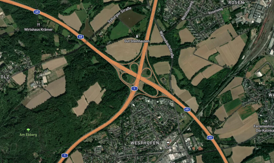
From all commercial traffic coming from the north and changing to the A45 at the Westhofen Kreuz, what amount drives through Lüdenscheid and what amount ends their trip in Lüdenscheid, during morning commute hours?
Figure 1. Weishofen Kreuz is the last decision point where drivers can decide to continue on the A45 south or not.
This is a concrete question that a traffic analyst might have to identify whether traffic follows the indicated traffic flow deviations (which typically keep through traffic on the highway), or whether drivers get off the highway and onto the smaller secondary roads.
Below we will work out this analytical question using the advanced space-time query language, and we will adapt it to eventually consider all traffic coming from the north and passing through the Westhofen Kreuz.
Step 6.1: A first advanced traffic flow filter
Let’s start with a simplified filter: Show all traffic leaving the A1 towards the A45 and driving to Lüdenscheid center.
In the advanced space-time query language, such a traffic flow filter is called an ASSET_ROUTE filter. But before we can use ASSET_ROUTE filters, we need to have areas available, as an ASSET_ROUTE describes which areas the traffic should flow through.
In our simplified query, we need at least 3 areas:
-
The area on the A1 north of the crossing
-
The area on the A45 south of the crossing
-
The area that corresponds to the center of Lüdenscheid
Drawing the areas of interest
Using the polygon controller at the top of the map, draw 3 shapes with following names:
-
A1N north of the crossing A1-A45 on the A1
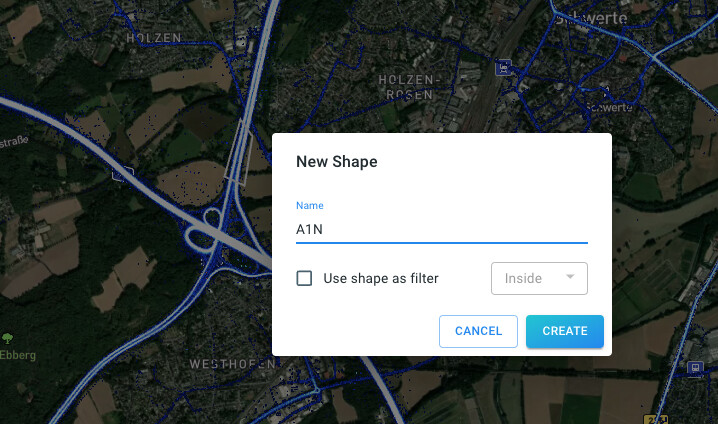 Figure 2. First polygon drawn north of the crossing on the A1: A1N.
 -
A45S south of the crossing A1-A45 on the A45
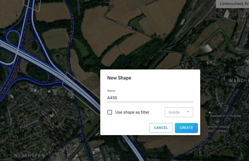 Figure 3. Second polygon drawn south of the crossing on the A45: A45S.
 -
Lüdenscheid around the center of Lüdenscheid
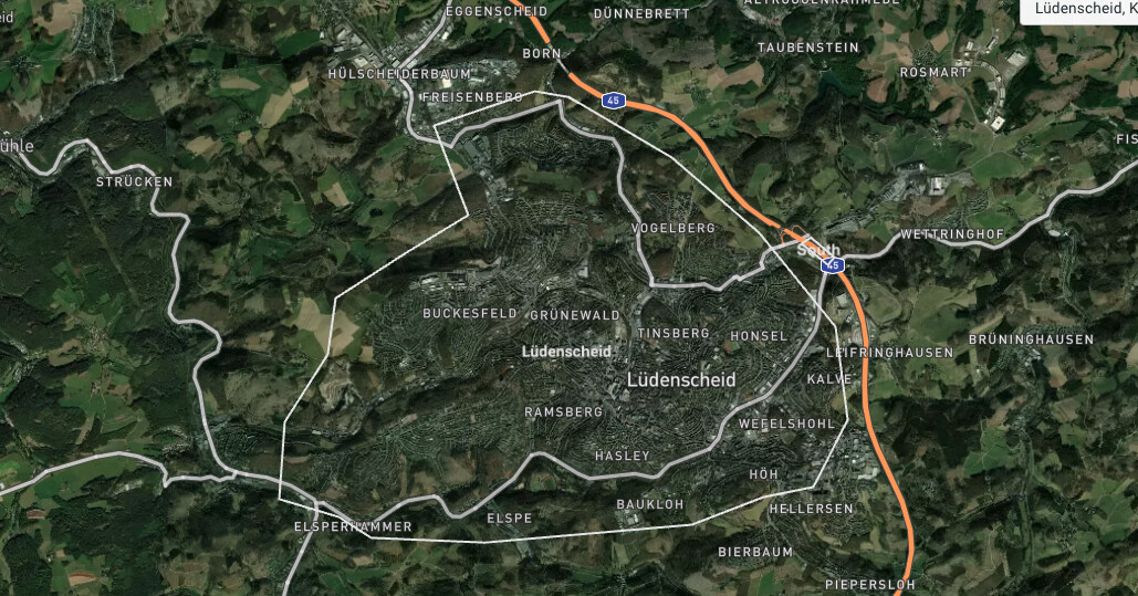 Figure 4. Third polygon drawn south of the crossing surrounding Lüdenscheid center: Lüdenscheid.
We will use these 3 shapes to build up our advanced traffic flow filter.
|
You can toggle the layer visibility of the |
Building the ASSET_ROUTE filter
Let’s incrementally build the filter to understand the different steps and concepts.
An ASSET_ROUTE filter describes which areas the asset (or in this case, a trip) should go through. It then matches all trips against the filter and retains the waypoints of the trips that match and that are inside the areas defined.
Given the A1N and A45S shapes, a first filter can look like this:
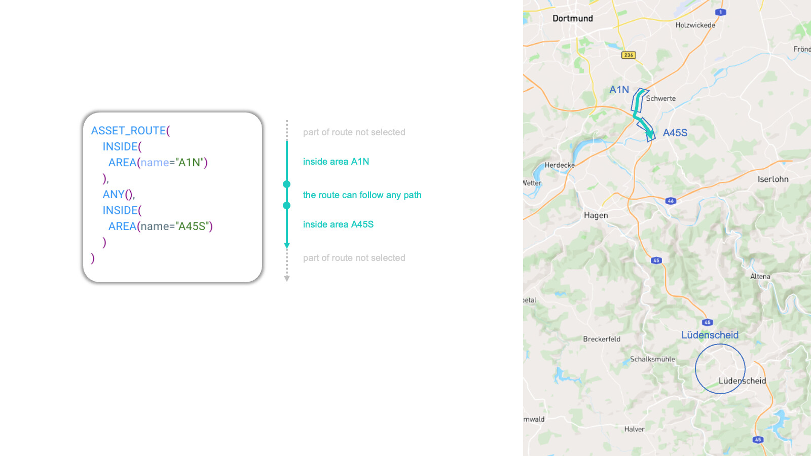
Figure 5. ASSET_ROUTE filter identifying trips coming from the A1 and driving onto the A45 south.
In the image above, we show 3 things:
-
On the left, the
ASSET_ROUTEfilter -
In the middle, next to the
ASSET_ROUTEfilter, a conceptual representation of a trip or route as it flows through the different stages of theASSET_ROUTE -
On the right, a visualization of the (part of) an asset’s route that complies with the filter, in blue.
In the following, we will use this representation to further build the filter.
Now, let’s apply the filter yourself:
-
Zoom in again on the A1-A45 crossing north of Lüdenscheid where you have drawn the two shapes A1N and A45S.
 Figure 6. Zooming in on the analysis area.
 -
Make sure the INRIX trips data layer is enabled and expanded in the LAYERS panel.
-
Click on the ADVANCED FILTER tab for the INRIX trips data layer
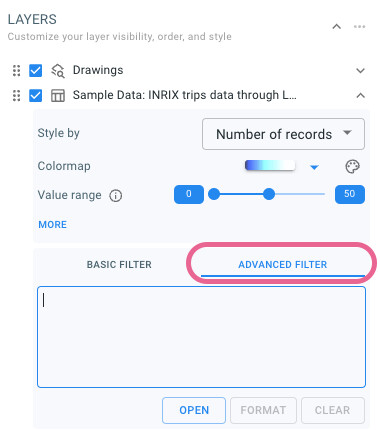 Figure 7. Advanced filter text editor.
 -
Type or copy-paste following
ASSET_ROUTEfilter in the ADVANCED FILTER text field.ASSET_ROUTE( INSIDE(AREA(name="A1N")), ANY(), INSIDE(AREA(name="A45S")) ) -
After a few seconds, the map, timeline and data distributions should update and only show the traffic that:
-
First is inside the A1N area (
INSIDE(AREA(name="A1N"))) -
Then can be ANYWHERE (
ANY()) -
And then should be inside the A45S area (
INSIDE(AREA(name="A45S")))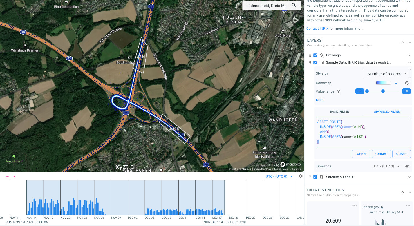 Figure 8. First advanced traffic flow filter applied.
-
This ASSET_ROUTE filter hence consists of 3 legs: a leg where the trip has to be inside A1N, then the trip can be anywhere, and then the trip has to be inside A45S. The platform will consider all trips in the data set and match them against these traffic flow conditions. It will then show only the parts of those trips that correspond to those 3 legs.
Note a few things about this filter:
-
It only shows the part of the trips that match the filter starting from when the trip enters A1N until the trip exits A45S. This means that for the matched trips, it does not show the entire trip.
-
It also shows traffic driving north on the A1N, then for example making a loop onto the A45 north of the crossing and then driving through the A45S area.
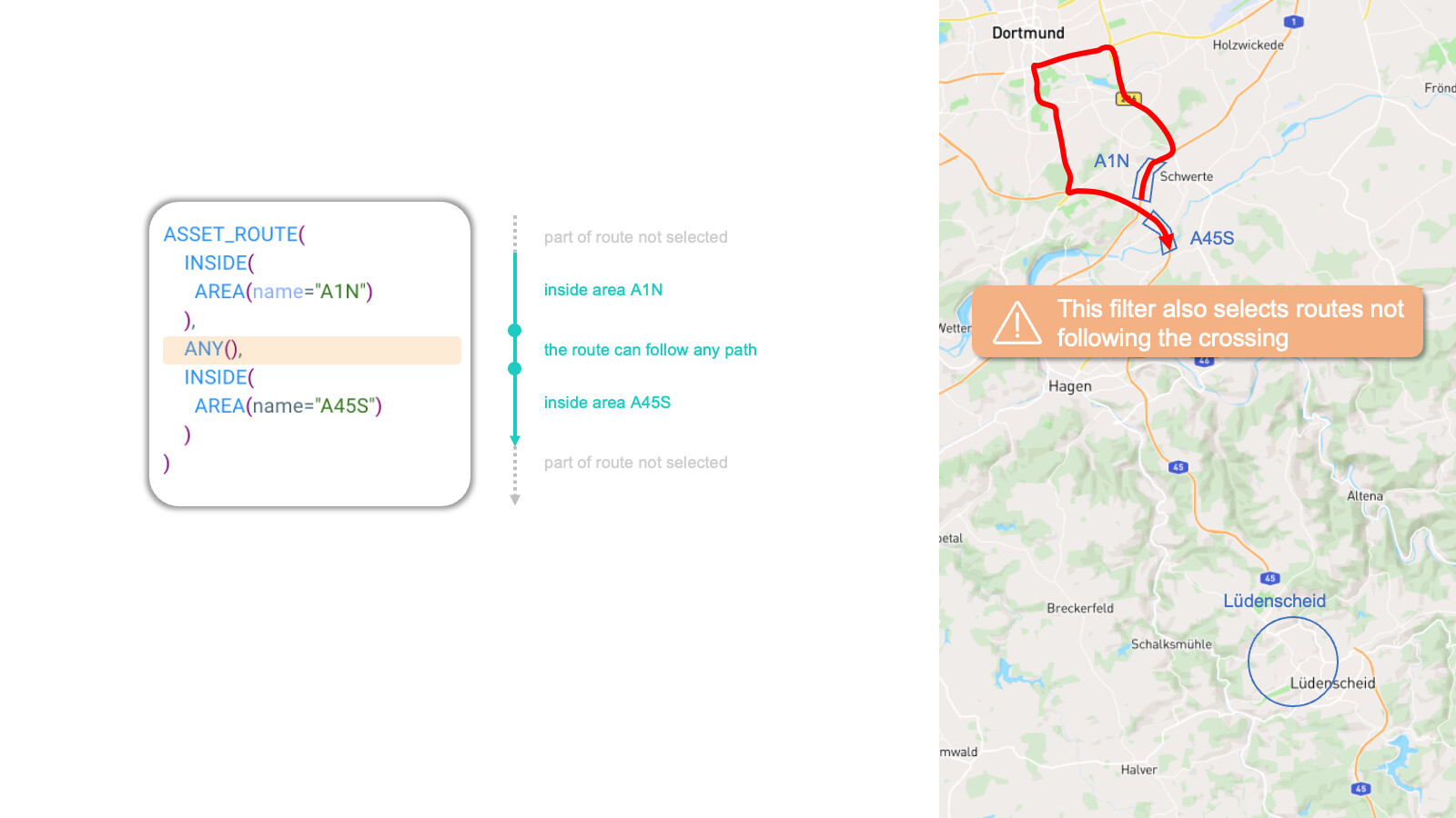 Figure 9. Trips also selected by our initial traffic flow filter.
In the next steps, we will modify our initial filter to rule out these trips driving north first, and to further consider only traffic driving towards the Lüdenscheid area.
|
Why is traffic flow filtering implemented using areas (polygons) and not using road segments (lines)?
In the above traffic flow filtering, we used polygons to denote the different areas we want the traffic to pass through. Why does the platform not use road segments? The reason is that area-based filtering is extremely flexible and it can be used to filter other traffic flows such as: traffic on a specific highway lane, pedestrians walking through a park, vessels sailing through the Atlantic, etc. You can however also use road segments as filters by creating an Areas of Interest layer by uploading a GeoJSON or SHP file with road segments (e.g., from OpenStreetMap). |
Step 6.2: Ruling out traffic driving north
Let’s first rule out the traffic driving north through A1N and only later through A45S, as we really want to see only the traffic that is driving south.
The easiest to rule out this traffic, is by replacing the ANY() part with a constraint that says that this leg of the trip has to stay on the crossing.
Follow these steps:
-
Draw a shape (e.g., a circle) centered on the crossing and overlapping the A1N and A45S areas.
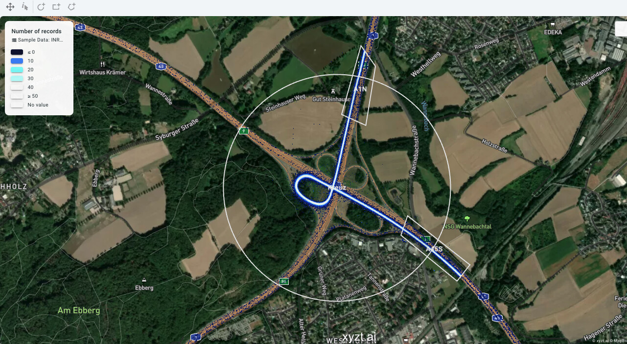 Figure 10. Drawing a circle named Kreuz covering the intersection.
 -
Name this shape Kreuz which is German for crossing.
-
Now modify the filter like this:
ASSET_ROUTE(
   INSIDE(AREA(name="A1N")),
   INSIDE(AREA(name="Kreuz")),
   INSIDE(AREA(name="A45S"))
)-
You should now see that the traffic north on the A1 disappears from the result.
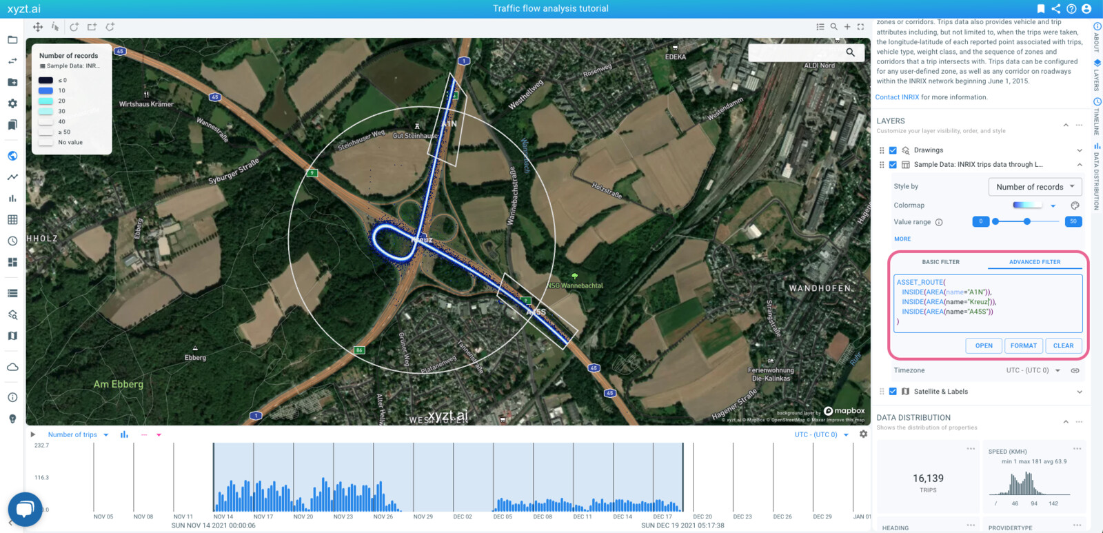 Figure 11. Traffic through A1N, Kreuz, and then A45S.
Conceptually, this is what the filter selects:
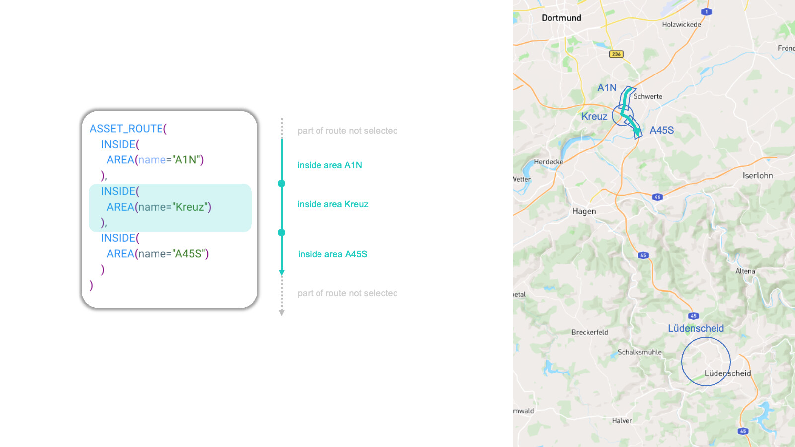
Figure 12. Conceptual representation of the traffic flow filter through A1N, Kreuz, and A45S.
Step 6.3: Extending the filter to account for traffic driving to Lüdenscheid center
Let’s look at our initial filter again: Show all traffic leaving the A1 towards the A45 and driving to Lüdenscheid center.
The above filter has selected the traffic changing from the A1 in the north to the A45 in the south of the crossing. We will now extend this filter to consider only the trips ending in Lüdenscheid center.
Follow these steps:
-
Add an
ANY()filter to account for the part of the trips after leaving the A45S area. -
Add a combined filter that says that the end of the trip has to be inside the Lüdenscheid polygon that you had drawn before.
-
This can be done using the
END()function which evaluates totruefor the last point of a trip, and -
The boolean combination function
AND(…)which can be used to combine multiple conditions.
-
-
The resulting filter looks like this:
ASSET_ROUTE(
   INSIDE(AREA(name="A1N")),
   INSIDE(AREA(name="Kreuz")),
   INSIDE(AREA(name="A45S")),
   ANY(),
   AND(
      INSIDE(AREA(name="Lüdenscheid")),
      END()
   )
)
Conceptually, this is what this filter describes:
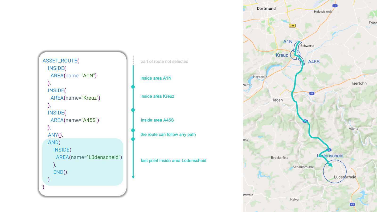
Figure 13. Conceptual representation of the traffic flow filter through A1N, Kreuz, and A45S, and ending in Lüdenscheid.
And this is what the traffic density looks like in the two weeks of December, after the closure of the highway. Note how traffic flows south on the A45 and then tries to find its way to the center of Lüdenscheid:
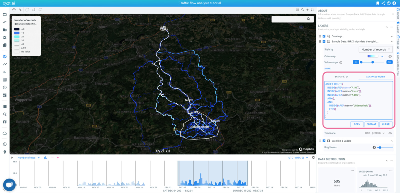
Figure 14. Traffic flow filter through A1N, Kreuz, and A45S, and ending in Lüdenscheid.
Step 6.4 Looking at traffic driving through Lüdenscheid
To obtain the traffic that flows through Lüdenscheid instead of ending in Lüdenscheid, we can simply modify our filter to:
ASSET_ROUTE(
   INSIDE(AREA(name="A1N")),
   INSIDE(AREA(name="Kreuz")),
   INSIDE(AREA(name="A45S")),
   ANY(),
   INSIDE(AREA(name="Lüdenscheid")),
   ANY(),
   AND(
      NOT(INSIDE(AREA(name="Lüdenscheid"))),
      END()
   )
)
Note that we added 2 more legs:
-
INSIDE(AREA(name="Lüdenscheid")), and -
ANY().
And modified the final leg to state that the end point of the trip should not be in Lüdenscheid:
AND(
   NOT(INSIDE(AREA(name="Lüdenscheid"))),
   END()
)
This is what the result looks like for the last two weeks of the data set:
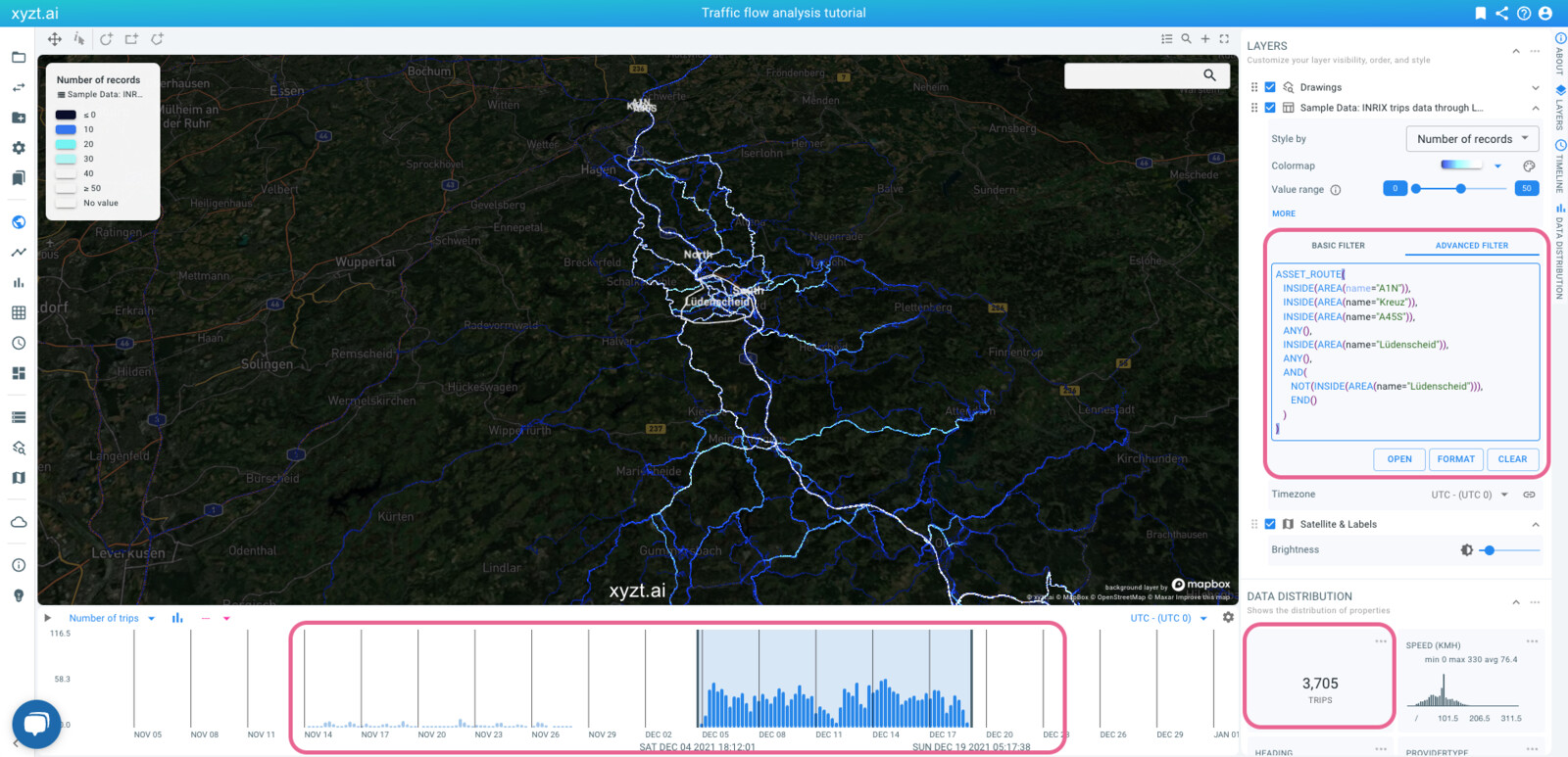
Figure 15. Traffic flow filter through A1N, Kreuz, and A45S, and through Lüdenscheid but ending outside Lüdenscheid.
Note a few things:
-
There are many more trips driving through than ending in the Lüdenscheid area*
-
There are many more trips following this pattern in the last two weeks (after the closure of the A45 highway), than before the closure.
Step 6.5 Comparing traffic flows with the split view capability
Let’s take our two filters (trips ending and trips driving through) and compare them side-by-side.
Follow these steps:
-
Click on the '+' button on the top-right of the map. This gives you two maps, initially with the same styling and filters.
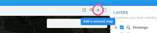 Figure 16. Adding a second map.
 -
Now click on the left map or on the MAP 1 tab in the LAYERS panel.
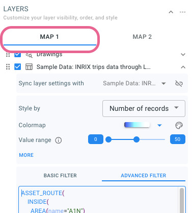 Figure 17. Focusing on the first map.
-
This makes the left map active, and allows us to modify the filter for the layer on this map.
-
-
Let’s revert the advanced filter for our INRIX trips layer on the left map to the traffic ending in Lüdenscheid:
ASSET_ROUTE(
   INSIDE(AREA(name="A1N")),
   INSIDE(AREA(name="Kreuz")),
   INSIDE(AREA(name="A45S")),
   ANY(),
   AND(
      INSIDE(AREA(name="Lüdenscheid")),
      END()
   )
)|
Working with two maps
When in split view mode, there are two maps, two timelines, two sets of data distribution widgets, and also two sets of layers. There is always one of two maps, timelines, etc. active. The active one can be identified by the active tab MAP 1 or MAP2 in the LAYERS panel or by the blue border at the top of the map and the bottom of the timeline. Toggling between the active map, timeline, etc. can be done by clicking on this tab in the LAYERS panel or by clicking on one of the maps and timelines. |
This is the result:
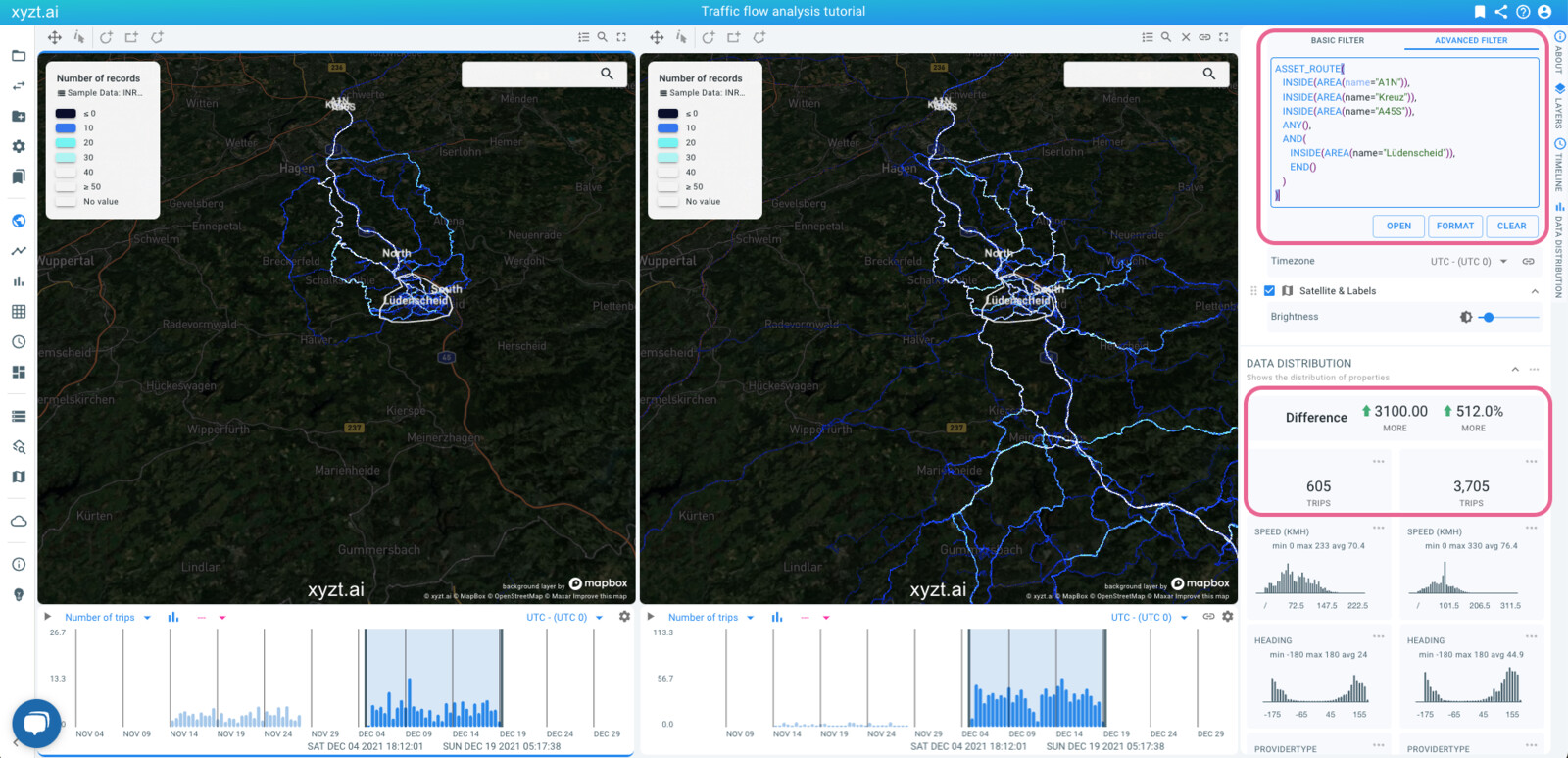
Figure 18. Left: traffic ending in Lüdenscheid. Right: traffic driving through Lüdenscheid.
Note how the left map and timeline update and now differ from the right map and timeline, as a different filter is set. Note also how you can compare the two filters in the DATA DISTRIBUTION part and see the difference in traffic. There is over 500% more through traffic than destination traffic coming from the A1 onto the A45 and through Lüdenscheid.
As a traffic analyst this will not make me happy, as it means that traffic diversions along the highways are not followed and drivers instead follow the smaller roads to make it through the Lüdenscheid area.
Step 6.6: Further extending our filters with ASSET and RECORD parts
By now you should understand how to filter on the flow of traffic. To also learn how to filter by asset or by record, let’s reconsider our initial traffic analysis question:
From all commercial traffic coming from the north and changing to the A45 at the Westhofen Kreuz, what amount drives through Lüdenscheid and what amount ends their trip in Lüdenscheid, during morning commute hours?
There are two parts we did not cover yet:
-
From all commercial traffic, and
-
during commute hours.
The first part, is called an ASSET filter: from all assets (i.e., trips in the INRIX terminology), we only want to consider the ones that are commercial. And since a car does not change from commercial to not commercial during a trip, this filter can entirely prune a trip if for example its start point is not flagged as commercial.
The second part, during commute hours, is a RECORD filter. From all the resulting (parts of) trips selected by the ASSET and ASSET_ROUTE filter, only select the records (waypoints in INRIX terminology, or GPS points), that have a time stamp during weekday morning commute.
The ASSET filter selecting only commercial traffic
The ASSET filter that selects only commercial traffic, for this data set looks like:
ASSET(
  EQ(
    START_PROP("ProviderType"),
    "2 fleet"
  )
)
This filter is read like this: From all assets (i.e., trips), take only the ones that have for the property with name ProviderType a value equal (EQ) to 2 fleet for their first record (START_PROP).
This is a very efficient filter, because we only have to look at the first record of all the trips and can immediately rule out the ones with a value 1 consumer, which is the other value that appears for this property.
To see this filter in action, follow these steps:
-
Reload the page and zoom in again on the Lüdenscheid area.
-
Copy-paste above filter in the ADVANCED FILTER text field.
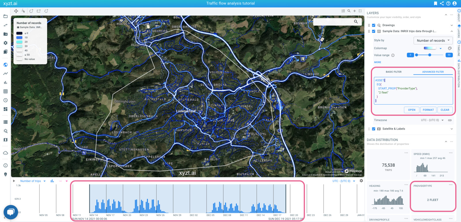
Figure 19. RECORD filter retaining only the fleet (commercial) traffic.
Notice how the DATA DISTRIBUTION widget for PROVIDERTYPE shows 2 FLEET. Also notice that there is slightly less fleet traffic during the highway closure compared to before, as can be seen on the timeline.
The RECORD filter selecting only the morning commute traffic
The record filter to only keep the records (i.e., waypoints) during morning commutes looks like this:
RECORD(
   AND(
     BETWEEN(
       HOUR(),
       6,
       10
     ),
     BETWEEN(
       WEEKDAY(),
       1,
       5
     )
   )
)
It says that:
-
It is a RECORD (
RECORD) filter, -
Following conditions should both be true (
AND(…)):-
The hour (
HOUR()) of the record should be between (BETWEEN(…)) 6am and 10am, and -
The day (
WEEKDAY()) of the record should be between (BETWEEN(…)) the first and fifth day of the week (i.e., from Monday through Friday).
-
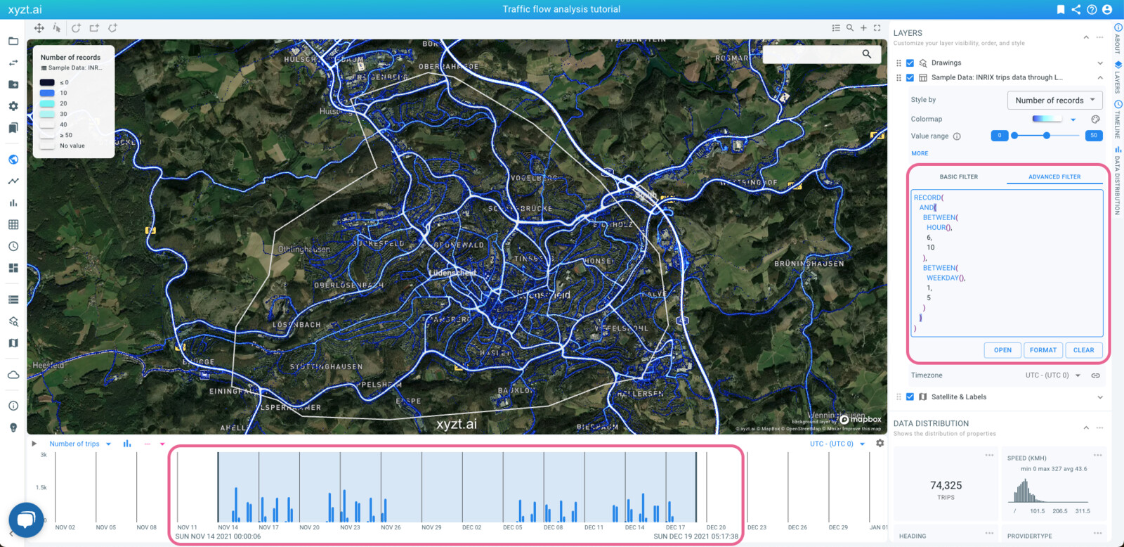
Figure 20. ASSET filter retaining only the morning commute traffic.
Combining ASSET, ASSET_ROUTE, and RECORD filters
Asset, asset route, and record filters can be combined using the pipe symbol, i.e. |.
For example: to obtain all commercial traffic leaving the A1 in the north and driving to the A45 south ending in Lüdenscheid, during morning commute hours, we obtain following filter:
ASSET(
  EQ(
    START_PROP("ProviderType"),
    "2 fleet"
  )
) |
ASSET_ROUTE(
    INSIDE(
      AREA(name="A1N")
    ),
    INSIDE(
      AREA(name="Kreuz")
    ),
    INSIDE(
      AREA(name="A45S")
    ),
    ANY(),
    AND(
      INSIDE(
        AREA(name="Lüdenscheid")
      ),
      END()
    )
) |
RECORD(
   AND(
     BETWEEN(
       HOUR(),
       6,
       10
     ),
     BETWEEN(
       WEEKDAY(),
       1,
       5
     )
   )
)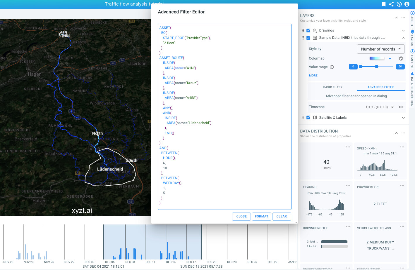
Figure 21. Combined ASSET, ASSET_ROUTE, and RECORD filter.
Step 6.7: Exercise
As an exercise: extend the filter to not only consider the traffic coming from the A1 towards the A45, but also the traffic that was already on the A45 and stays on the A45.
|
Draw an additional polygon named |
Next part
Go to the next part: Further reading
Got feedback? Additional questions? Just want to have a friendly chat?
Get in touch!