Got feedback? Additional questions? Just want to have a friendly chat?
Get in touch!
What’s New?
June 2026
-
Distribution exports have been improved to make the reported values easier to interpret and validate. In addition to the existing ratio columns, distribution exports now also include the absolute number of records for each value or interval.
This applies to both the frontend download exports and the public API output. For area-based distribution exports, the existing ratio columns remain in their original position for compatibility, and the new record-count columns are appended after them.
No-data values are now also included more consistently in distribution exports. When records without a value are present, an additional no-data row is included with both its ratio and absolute record count. This makes the exported totals complete and ensures that the reported ratios add up correctly, also when part of the data has no value for the selected property.
-
Various improvements have been made to the Trajectories and Realtime visualization modes for Movement data sets. Tooltips now show the timestamp, longitude, and latitude. Clicking a trajectory line or icon now copies the tooltip contents to the clipboard. When icon tracing is enabled, an icon is now also shown at the filter’s maximum time.
-
The scale indicator now supports both metric and imperial units.
-
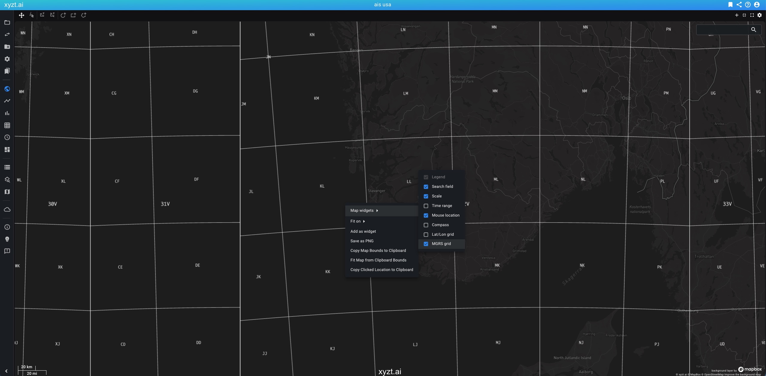
We have added 3 new map widgets: a time range indicator, a mouse location indicator, and a compass widget. The compass widget lets you reset the map to north-up orientation. All map widgets can now be toggled from a single settings menu, available under the gear icon in the top-right corner of the map.
-
You can now enable a longitude/latitude grid or a MGRS grid on spatial maps for additional situational awareness.
These overlays make it easier to estimate positions, communicate locations, and interpret map data in operational or geospatial workflows. The longitude/latitude grid is useful for general geographic reference, while the MGRS grid supports military, emergency response, and other coordinate-based field operations.
May 2026
-
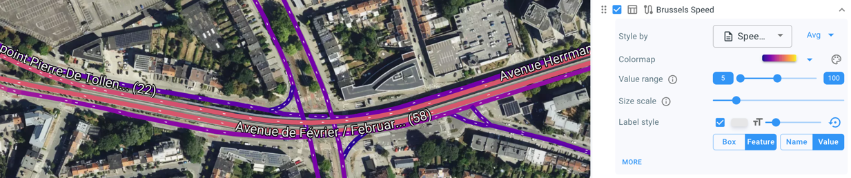
You can now configure label placement and label detail for Geometry, Time Series, and Movement Path data set layers. Label placement lets you choose between callout boxes and on-feature labels. Label detail lets you choose whether to show only the display name, or the display name together with the active style-by value.
-
On-feature labels for line features can now follow the shape of the line. This makes it possible to render street-style labels directly along roads, routes, and other line geometries.
-
Added record count histograms for native time series data sets, available on both the Visual Analytics and Trend Analytics pages. These show the number of records per time bucket, complementing the existing asset count histograms. This is useful for traffic counting stations, where each vehicle passage is stored as a separate record, or maritime anchorage zones, where each registered vessel presence can be counted over time.
-
Added a REST API endpoint to render a project bookmark map as a PNG image:
GET /public/api/projects/{projectId}/bookmarks/{bookmarkId}/map. External systems, reports, automations, and agentic workflows can now generate map snapshots directly from saved bookmark state and requested map bounds, without requiring interactive use of the UI. Refer to the API documentation for capabilities and limitations.
April 2026
-
WMS background layers now automatically refresh every 10 seconds, so dynamic map data stays up to date.
-
WMS layer URLs now support the
STYLES="…"parameter, allowing the correct server-side style to be selected. -
Dashboards now support a flexible grid layout, letting you place multiple smaller widgets alongside a larger one — for example, two half-height widgets next to a full-height one. Drag and resize widgets directly from the dashboard page.
-
Default flow placement: newly created widgets are automatically placed at the next available position in the grid.
-
Explicit positioning: drag a widget to pin it to a specific position. Via the API, you can also provide explicit grid coordinates alongside the widget’s width and height. If the target area is already occupied, the widget falls back to automatic placement.
Existing dashboards are not affected and continue to use the previous layout.
-
-
You can now replace the data set with a compatible one on any project attachment while keeping all widgets and saved bookmarks intact. A compatible data set is a data set of the same type with the same properties, but potentially with different data.
-
We have introduced managed data sets — a new concept that wraps a regular (source) data set and adds a layer of indirection on top of it.
-
Update once, reflect everywhere: because a managed data set points to a source data set, changing that source immediately updates every project that uses the managed data set, across all users — no manual re-attachment needed.
-
Attach the same source multiple times: you can create several managed data sets backed by the same source and attach them independently to the same project, each with its own styling, filtering, and configuration.
-
-
Percentile aggregation is now available for map and route analysis styling. In addition to existing modes (min, max, avg, sum, mode), you can now select any percentile from P5 to P100, including a dedicated median, to color data by the statistical distribution of the record values.
-
Improved Parquet support for nested data. You can now define nested Parquet properties in the data properties file using dot notation, such as
device.id,point.x, orpoints.ts.
February 2026
-
Long descriptions for projects, data sets, area of interest layers, and background layers are now collapsed by default. Click
MOREto expand and view the full description.
January 2026
-
Added Year as a bucket option for categorized trend analytics. We also simplified the chart label formatting for Hour, Day, and Month views.
-
You can now customize the colors of the dwell time charts.
-
You can now compute total dwell times next to average and individual dwell times. This enables you to analyze the total time spent in different areas.
December 2025
-
You can now save the data on the map for Geometry data, Time series data, and Movement path data as GeoJSON. This enables you for instance to compute a density map of traffic on a road network and then use the result for further analysis or visualization in other tools.
-
You can now restore a copied map bounds from the clipboard in the visual analytics page. This allows you to fit the map on a previously saved map bounds. You can find the action in the context menu that appears when right-clicking on the map.
November 2025
-
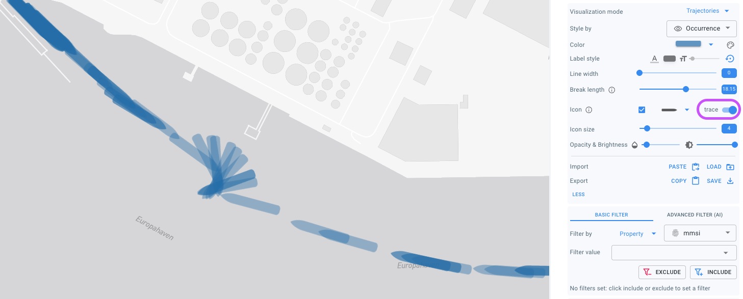
When using the trajectory visualization mode, you can now display the entire movement trace, not only as a line, but also using icons at all recorded positions instead of just the most recent one. This makes it easy to analyze the swept path of vehicles or vessels along their route.
You can now find a trace toggle button for this.
-
Movement data sets that use the real-time visualization mode, now show hover labels and regular labels consistent with the trajectories visualization mode.
October 2025
-
Data sets can now be cleared using a REST API call. This means that uploaded files and the corresponding processed data can be removed while maintaining the data set configuration. See the
/datasets/{dataSetId}/clearend point. -
Improved date-time picker for absolute time configuration: You can now select the day, month, and year using drop-down boxes, with available options automatically hinting to the time range of your project’s data sets. In addition, it’s now easier to align your selection with the start or end of a day. You can toggle to a text field input, for instance to copy-paste date-time values.
-
The Database Module now supports Movement Path data in addition to Geometry and Time Series data. Similar to the native movement path data support, you first create a Geometry data set based on a geometry table in your database. You then create a movement path data set, based on an additional data (containing trips info) and optional metadata table.
-
The Database Module now supports ClickHouse, a high-performance analytical database. Similarly to Postgres, this database supports Geometry, Time Series, and now also Movement Path data sets.
-
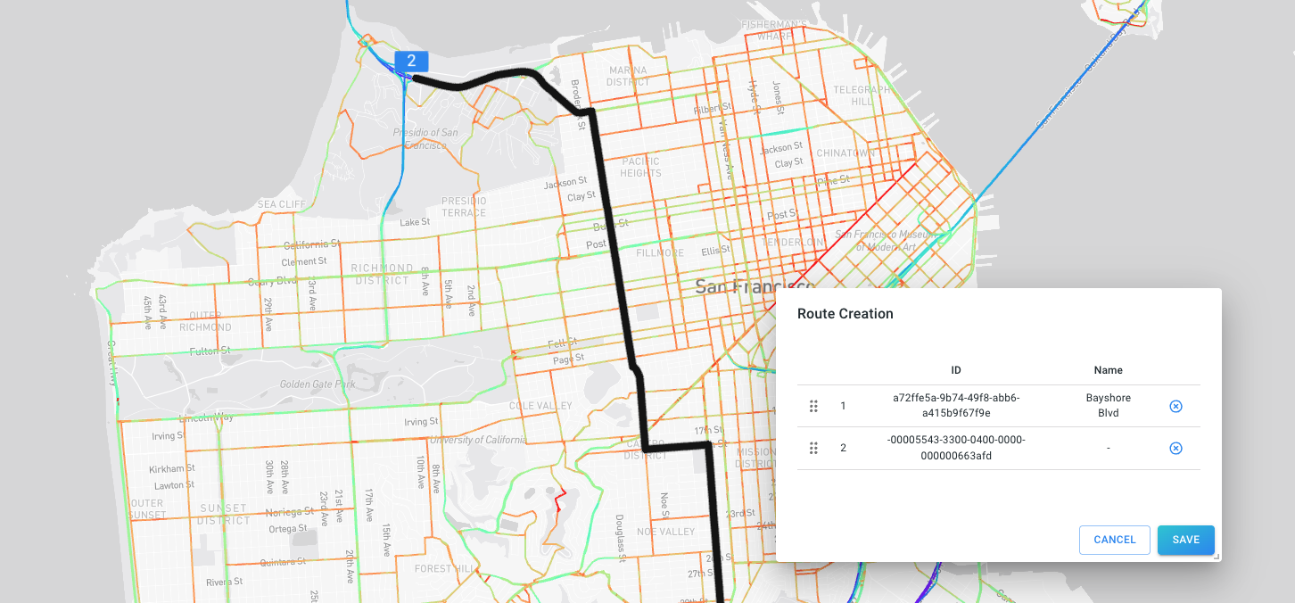
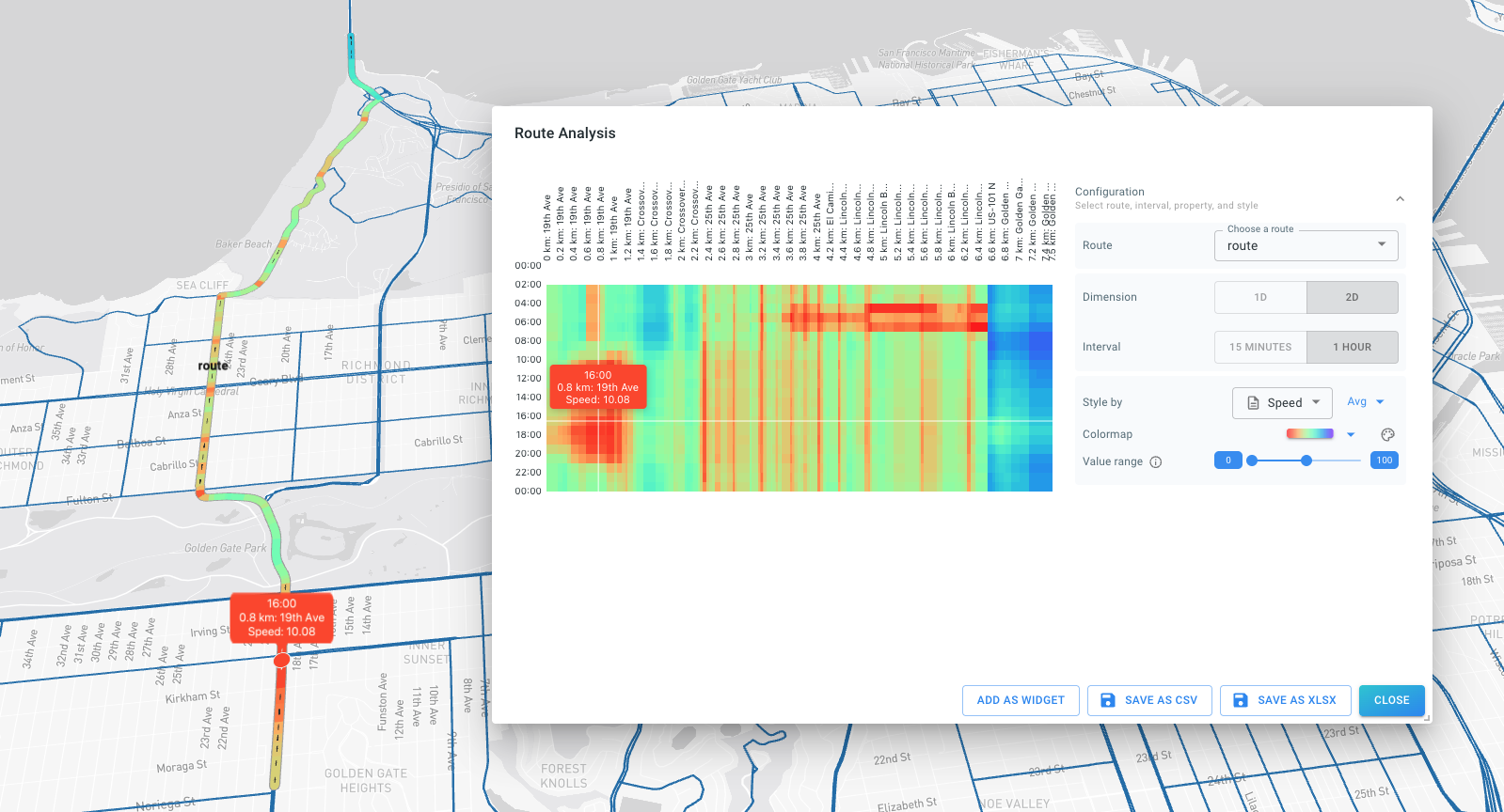
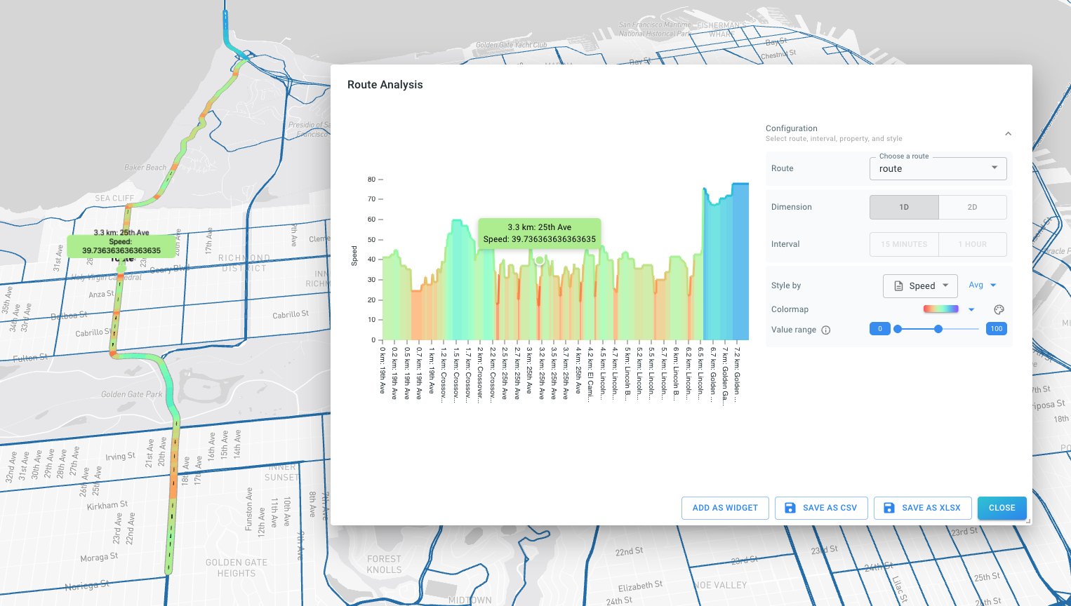
Various improvements have been made to the Network Route Analysis Module: You can now style the computed diagrams separately from the corresponding layer. You can now also perform route analysis on database movement path data sets.
-
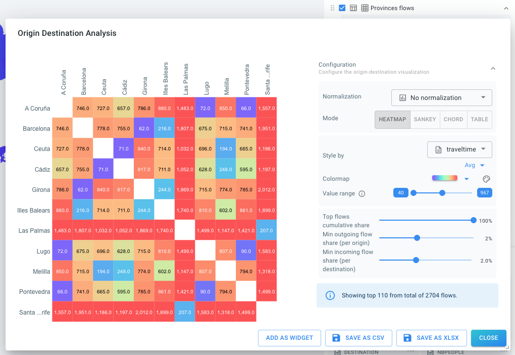
Various improvements have been made to the origin-destination analytics capability. You can now work with pre-computed origin-destination data in database time series data sets. Select Origin and Destination to configure the corresponding data properties/columns. The origin-destination analysis can then be used from the Visual Analytics page by clicking on the matrix icon next to the layer’s name.
September 2025
-
Geometry, Time Series, and Movement Path layers now use an improved label deconfliction algorithm resulting in better label selection and more consistent placement.
-
There are two new default color maps named
stoplight(green to yellow to red) andstoplight2(red to yellow to green) that are useful for instance to style speed on road segments.
August 2025
-
* You can now use (XYZ) tiles web maps as background layers. XYZ tiles are a common way to provide multi-level tiled map data using a URL of the form
http://…/Z/Y/X.pngor similar. For example,https://services.arcgisonline.com/ArcGIS/rest/services/World_Street_Map/MapServer/tile/{z}/{y}/{x}, provided by ESRI, serves a world street map background layer. -
We’ve doubled the default capacity (memory and compute cores) on our cloud deployment. This upgrade delivers faster analytics performance, especially when working with very large data sets.
-
The Categorized Trend Analytics page now supports three new bucket strategies:
Hour,Day, andMonth. These allow you to create continuous, time-aligned buckets exactly on the hour, day, or month boundaries. This is different from the existing modes likeHours of Day, which group data by clock hour (e.g., all events from 14:00–14:59, regardless of date).Use case: Want to analyze how traffic evolved hour by hour over multiple days? Use the
Hourmode to precisely align buckets to each hour and track patterns without aggregation across different dates. -
We’ve also resolved a small alignment issue in the
AutoandFixed bucket sizemodes. Previously, buckets could sometimes be slightly misaligned with the start of your selected time period. This has now been fixed for more accurate trend visualizations.
June 2025
-
You can now configure the color of the timeline on the Visual Analytics page and when used as a widget. Click the three dots in the top right corner of the timeline and select Edit > Chart Style. Both properties can be customized individually.
-
You can now configure the chart colors in regular trend analytics and their widgets. Click the three dots in the top right corner of the chart card and select Edit > Chart Style. You can customize the main chart color and the difference colors when comparing two time periods.
-
You can now configure the chart colors in categorized trend analytics and their widgets. Click the three dots in the top right corner of the chart card and select Edit > Chart Colors. Each category can be styled individually.
-
You can now enable linear interpolation for charts and their widgets on the timeline in the Visual Analytics page and on the regular Trend Analytics page. This fills gaps between data points to create a more continuous chart. For example, if your time series data has measurements only every hour, the values will be connected using lines or linearly interpolated bars, depending on the chart type. Click the three dots in the top right corner of the chart card and select Edit > Chart Style.
April 2025
-
There are three new optional modules:
-
The Database Module enables direct connection to a database. Specify the URL of the database and the table names you wish to use. The platform will directly visualize and analyze the data, eliminating the need for a data import in the platform. Currently, PostgreSQL with the PostGIS extension is supported as a database. The module supports both Geometry and Time Series data sets.
-
The OGC WMS Server Module facilitates the integration of xyzt.ai maps within compatible GIS applications, such as ArcGIS and QGIS. It allows for direct integration of xyzt.ai layers, supporting both Geometry, Time Series, and Movement Path data sets.
-
The Network Route Analysis Module allows to construct routes along a graph (road network) including the creation of distance-time (TX) diagrams.
For further information and to explore these optional modules, please reach out to sales@xyzt.ai.
-
March 2025
-
The visual analytics page now displays a scale indicator in the lower left corner of the map.
February 2025
-
You can now use SHP files to define the geometry for Geometry data and Time series data sets, alongside GeoJSON data. Since SHP files consist of multiple files, they must be zipped before upload. You can either upload multiple zip files or include multiple SHP files in a single zip file.
-
For Areas of interest and Background layers, you can now also upload zip files containing multiple SHP files.
-
GeoJSON data has been renamed to Geometry data in both the web application and the REST API.
-
A new tutorial to learn how to upload INRIX Trip Paths data was added.
-
The origin-destination analysis now includes a table view for computed results, in addition to the matrix representation. The table can be sorted by number of trips, travel time, and other metrics. It also supports matrices larger than 100x100 and can be added as a widget on the dashboard.
-
When creating projects with multiple data sets, only the first data set is now visible by default. You can adjust the visibility and create a default bookmark to customize the project’s default opening behavior.
January 2025
-
A new data type has been added: Movement path data. This data type enables the representation and analysis of trips following road networks. It allows for detailed street analysis, traffic flow analysis, origin-destination analysis much like the already existing Movement data.
Movement path data consists of (map-matched) trips defined by a series of road segments. While movement data consists of trips defined by a series of GPS coordinates. The former is often a more natural data representation for analysing road traffic.
To work with movement path data, you first need a geometry data set consisting of road segments, ideally with a property that defines the Road class for multi-scale road network handling. Next you need data files (in CSV or Parquet) that represent the sequence of road segments traveled by all trips. Each entry in the data files represents a part of a trip, referencing the trip by its ID and referencing the road segment by its ID. Next, you can also add metadata for the trips (as CSV or Parquet) files, where each entry in those files references a trip by its ID. The data files typically contain time-varying properties such as speed. The metadata files typically contain constant properties such as vehicle type.
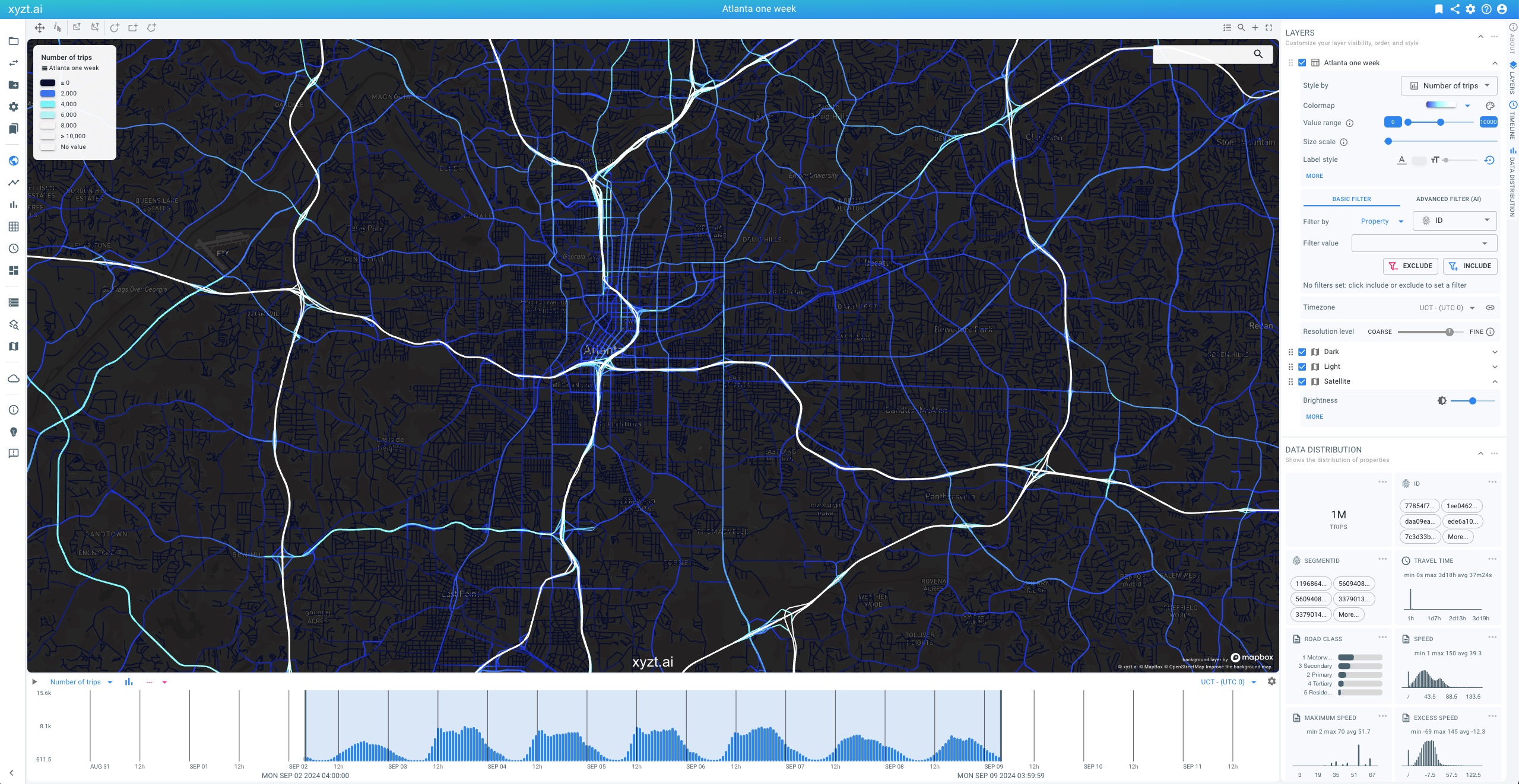 Figure 1. Example movement path data set from INRIX consisting of trips along a road network.
A prominent example of movement path data in the traffic/mobility industry is INRIX Trip Paths data.
A new tutorial to learn about movement path data was added.
-
Time series, Geometry, and Movement path data now use a multi-scale approach when handling road segment data. If your data set has a property with special meaning Priority Level with values (starting with) a number from 1 to 9 where 1 corresponds to the most important road type (e.g., highways), an automatic multi-scale representation will be generated. The approach favors larger roads (i.e., priority level 1) when zoomed out and smaller roads (e.g., priority level 6 or more) when zoomed in. This enables you to use country-wide road networks in your analysis.
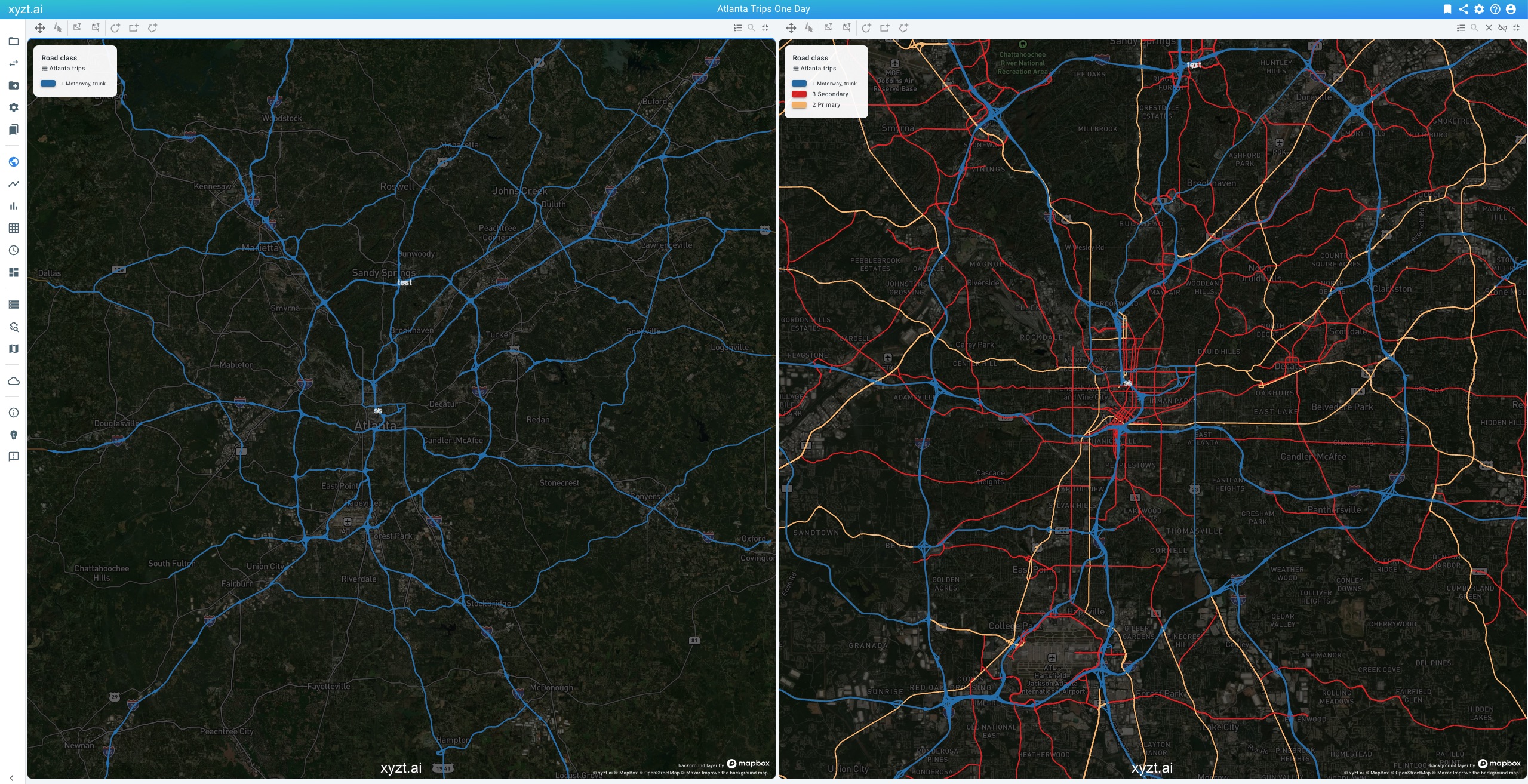 Figure 2. Multi-scale handling of road network data. Left; Only showing the motorways when zoomed out. Right: also showing the smaller roads when zooming in.
 -
Time series, Geometry, and Movement path data now enable the analysis of two-way roads. If your data set has a property with special meaning Reverse ID, the platform automatically understands that the road is a two-way road. For instance, if the identifier of a road segment is
2014921_0, then the reverse identifier might be-2014921_0. When configuring the reverse identifier, the platform understands that the road segment needs to be handled (and visualized) as a two-way road.Your temporal data (for time series sets) and movement data (for movement data sets) can then represent data for both sides of the road by using either of the two IDs (
2014921_0or-2014921_0in the example above).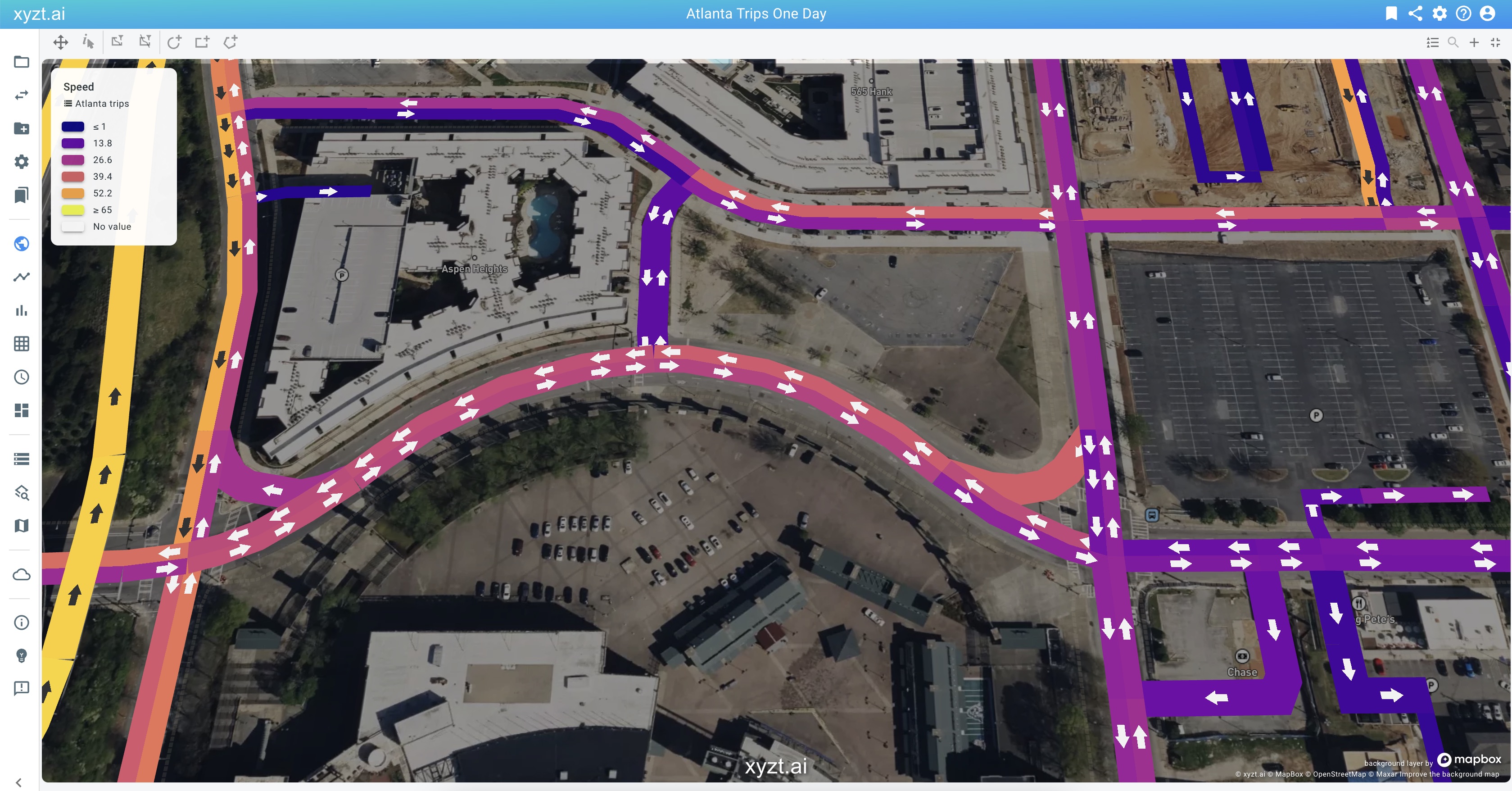 Figure 3. Handling of two-way roads, with indication of driving direction.
 -
Road networks defined in Time series, Geometry, and Movement path data sets now display an arrow pointing in the driving direction when the road is visualized sufficiently widely. This benefits analysis of traffic on bi-directional roads. You can change the width of the visualized road segments using the Size scale slider.
-
Time series and geometry data sets now use the 'Style by' value as label instead of the shape’s name. This enables faster insight generation and more informative visualization. For instance, when displaying speed on a road segment, the label will now show the (average/min/max/…) speed in the label. Additional information is now also shown when hovering with the mouse.
-
Time series and geometry data sets now do not expose the shapes as areas of interest shapes by default. You now have to explicitly configure this. When disabled, you cannot select the shapes as areas on the different analytics pages, for instance to display multiple trends on the Trend Analytics page. If enabled, you can use the shapes in the data set as before as areas of interest shapes.
-
Labels for Time series, Geometry, and Movement path data sets are now deconflicted (decluttered) for a better visual representation.
-
Some of the default styling options have changed. Styling by a numeric property now selects the Rainbow colormap by default. Accumulation styling is now also disabled by default. The latter can be enabled to apply a density effect based on the number of records or assets, in addition to the colormap used for styling.
October 2024
-
Experience the power of natural language interaction with the Just ask xyzt.ai™ beta program. Effortlessly set advanced space-time filters by simply asking a question—no complex query building required. Let AI handle the details, so you can focus on gaining insights faster and with greater ease. Want to join the beta? Contact support to get started today.
September 2024
-
You can now edit and replace widgets on the dashboard. To modify an existing widget, click on it, make your changes on the page, then select Add as widget…. Choose REPLACE and select the widget you want to update from the drop-down list. You can also replace a widget with an entirely different one (e.g., switching a visual analytics widget for a trend analytics widget).
-
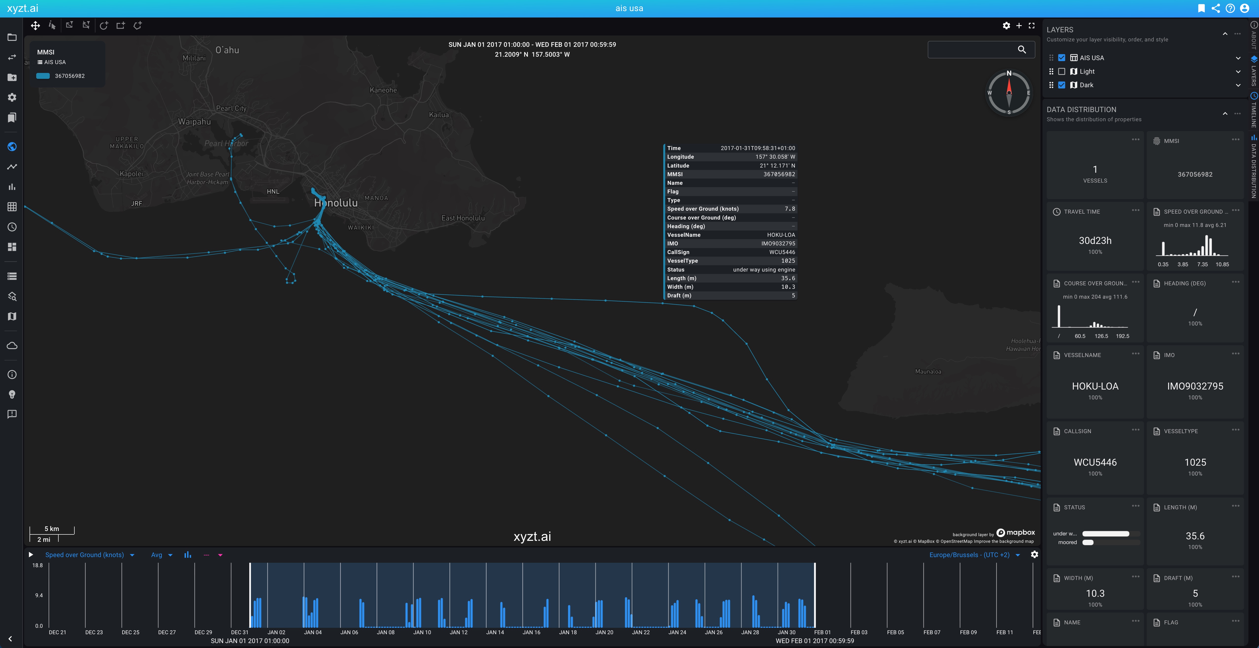
Travel Time is now a derived property available in Movement Data sets. It represents the time difference between the end and start of an asset’s journey.
If no filtering is applied, Travel Time is the difference between the last and first recorded data points of the asset. When a route is specified, such as
ASSET_ROUTE(INSIDE(AREA(name="New York")), ANY(), INSIDE(AREA(name="Boston"))), the travel time is the difference between the last and first records along that defined path (i.e., the last record in the Boston area and the first in the New York area).This new feature is available on the Visual Analytics page (Timeline and Data Distribution Panel) as well as on the Trend Analytics and Distribution Analytics pages. Users can now analyze key metrics such as average, min, max, and mean travel times, along with changes and distributions of travel times.
Travel time is automatically included in both new and existing movement datasets. For more details, refer to the dedicated article Travel Time.
-
Categorized Trend Analytics now supports the creation of custom categories. In addition to categorizing based on data properties, time periods, or areas, users can now build categories using complex filters.
For instance, you can analyze trends along multiple routes in a road network by defining different
ASSET_ROUTEfilters, for instance to compare travel time changes across these routes. This feature also allows for more flexible analysis by combining data properties. For example, you can create one option forLightandMediumvehicles, and another forHeavyvehicles, enabling more customized comparisons and insights. -
The Categorized Trend Analytics page now requires defining a Spatial Query Region to limit the search area when computing trends. This ensures that analytics are focused on a specific area of interest, such as a highway intersection or a port terminal, and prevents unintentional use of the entire dataset region.
For Movement Data, note that the larger the computation area, the lower the resolution. Therefore, it is recommended to define the spatial query region as small as possible to maintain higher accuracy and performance.
-
The Categorized Trend Analytics feature now includes configurable Calculation Modes, offering a distinction between record-based and asset-based calculations.
When analyzing trends over time, records (from different assets) that fall into the same time interval can now be combined in various ways. Additionally, when calculating trends by hour of the day, day of the week, month of year, the method for combining values is fully customizable.
See this article for more details on the calculation modes.
-
You can configure a default timezone on the project. This timezone will be used by default on any of the analytics pages when you open that page for the first time.
August 2024
-
The platform now supports a new data set type: Point Data. This type includes datasets composed of independent, unrelated measurements, each associated with a specific location. Examples include driving events such as harsh breaking, cornering,… For more details about the different types of datasets supported by the platform, please refer to the Different types of data sets article.
-
You can now use Parquet files in your data sets, whereas previously only CSV files were supported. The Different types of data sets article provides a list of supported file formats for each dataset type.
-
When defining the structure of a new data set through the wizard, you can now upload an example file and define the different properties from the uploaded file. Read the Auto-detection of the data properties article for more information.
-
For movement data sets, you can now enable labels for trajectories with icons. This enables you to more easily identify assets such as vessels moving on the map, e.g., showing the vessel’s MMSI identification number. In addition, you will now see a tooltip with all the record properties when moving with the mouse over a trajectory line or the associated icon.
-
You can now specify a start and/or end time on the origin-destination analytics page.
July 2024
-
Widgets for dwell time and trend analytics now are sized responsively on the dashboard. Also various improvements were made to the categorized dwell time charts, including addition of titles, time ranges, and a legend consistent with the other charts.
-
All chart data can now be downloaded also as Excel files (.xlsx). This has the benefit over CSV files that the data can easily be opened in Excel with proper column layout and character formatting. Right-click on the chart, or on the three dots to find the new download functionality.
-
The vertical axis (y-axis) of the Visual Analytics timeline charts and the Trend Analytics charts can now be configured to a fixed range, for example, always showing number of assets on a scale from 0 to 1000. Click on the three dots and choose Edit.
Using fixed vertical ranges has the benefit that you can place multiple charts side by side on a dashboard and allow for easy visual comparison.
-
You can now create a new data set by initializing it from the settings of an already existing data set. This means that the new data set takes all data (and metadata) properties and all configuration settings.
This has the benefit that uploading similar data sets requires less setup.
-
Performance of Origin-Destination and other route-related computations has been improved. Note also that the Origin-Destination analytics now defaults to "Strict From" and "Strict To".
-
You can now save and load layer styles on the Visual Analytics page. This enables you to configure styling once and re-use the same styling configuration for a compatible data set. Compatible data sets are data sets with the same data properties.
You can find the buttons to export and import layer styles in the layer styles panel by clicking on MORE.
-
The advanced filter editor has been extended with improved syntax error highlighting, auto-completion, and adaptive documentation pointers.
When opening the dialog, there is now also UI that can be used to select and insert data properties, property values, and areas.
February 2024
-
You can now define one or more categories on the Trend Analytics page. This enables you to analyze and download trends divided in subgroups, e.g., by a property, or by different areas, or by logical time units. Choose Categorized as the mode on the Trend Analytics page.
-
You can now choose German, French, Spanish, and Dutch, next to English as the language.
-
We have added several new tutorials:
-
A new tutorial on how to upload INRIX trips data.
-
A new tutorial on how to analyze traffic flows using floating vehicle data.
-
A new tutorial on how to automate data uploads and other platform actions using the REST API and Python.
-
-
There is now a compact view for the projects, data sets, data stores, areas of interest, and background overview pages. You can toggle by clicking on the table icon at the top of the respective pages.
Got feedback? Additional questions? Just want to have a friendly chat?
Get in touch!